- Review: found
Review of 'Statistical Analysis of Numerical Preclinical Radiobiological Data'
Average rating: | Rated 3.5 of 5. |
Level of importance: | Rated 3 of 5. |
Level of validity: | Rated 4 of 5. |
Level of completeness: | Rated 2 of 5. |
Level of comprehensibility: | Rated 4 of 5. |
Competing interests: | None |
Reviewed article

- Record: found
- Abstract: found
- Article: found
Statistical Analysis of Numerical Preclinical Radiobiological Data
Review information
Review text
Introduction
This review reports the results of attempts to reproduce the findings presented by Joel H. Pitt and Helene Z. Hill in the paper “Statistical analysis of numerical preclinical radiobiological data,” published in ScienceOpen Research in January 2016. We thank the authors for making their data public and for publishing in an open journal, both of which made the work we present in this review possible. We comment on the strengths and potential areas of improvement of the aforementioned paper, based on our experience in replicating the reported results. In addition, we offer suggestions for improving the statistical analyses and computational reproducibility of said paper, including questions and potential issues that arose in our re-analysis of the data. We note that this review was vetted by Philip B. Stark – and, accordingly, are thankful for the commentary he provided; still, we emphasize that the work and opinions found in the present review are those of the authors alone. Further, we would like to add that the authors – Nima Hejazi, Courtney Schiffman, and Xiaonan Zhou – all contributed equally to the work that led to the production of this review. Finally, in keeping with the goal of reproducible research, all of our work, largely in the form of Jupyter notebooks, is publicly available on GitHub at https://github.com/nhejazi/stat215a-journal-review; we welcome independent review and commentary.
In the paper, the analyses reported by Pitt and Hill appear to be motivated by the belief that a single investigator (RTS) in one of the labs studied reported false, fabricated colony and Coulter counts in radiobological data from a preclinical study. How the authors came to harbor such a suspicion is, to our understanding, never made entirely clear (e.g., were they exploring the data, did they hear a tip from a colleague). To test their suspicion in a manner more rigorous than simply plotting and comparing distributions of counts and mid-ratios, the authors carried out several hypothesis tests against null hypotheses that would hold if the data were not fabricated. For example, the authors assert that, if the data were produced honestly, the distribution of terminal digits in the Coulter counts would be uniform and that the number of triples containing their own means should be limited. Such null hypotheses were based on the authors’ speculations as to how data would be fabricated (e.g., start by choosing a mean value then subtract and add some value from the mean) and how counts would be generated if they were the result of true biological processes (e.g., independently with equally likely digits).
To carry out tests examining the means of the observed count triples, the authors assumed that each independent triple was composed of a set of three I.I.D. Poisson random variables. In settings where the number of successes found in independent trials was being tested (as in the case of the number of equal terminal digits), the authors used the binomial distribution; to test for a supposed multinomial distribution, they used the well-known chi-square goodness of fit test. In employing these well-known statistical tests, the authors were able to present a probabilistic perspective as to whether the data were fabricated. All tests performed by the authors suggest that the investigator of interest (RTS) fabricated at least some data.
Replication of Results
In keeping with the ideal of computational reproducibility, accuracy and honesty in academic research – motivations of the original authors themselves – we sought to reproduce many of the data summaries and analyses reported in the paper by Pitt & Hill. The vast majority of our analyses were performed using the Python programming language (v.3.5). We were able to reproduce Table 1 using the formula for the probability that a triple of I.I.D. Poisson random variables contain their own mean, found in the appendix of the original paper. We did not check the proof of the formulation of the probability, but we were able to very nearly computationally replicate the results reported from use of said equation. Next, we attempted to replicate Table 2; however, some of the reported values for complete, total and mean-containing triples we found differ from those presented in the paper (see Table [table1] of this review and Table 2 of the original paper). For example, the authors of the paper report 1, 716 complete triples, 1, 717 total triple and 173 mean-containing triples for the RTS Coulter data set. This is at odds with the 1, 726 complete triples, 1, 727 total triples and 176 mean-containing triples we found in the RTS Coulter data set. Despite this, we believe our summaries of the RTS Coulter counts to be consistent with the data set. The Excel spreadsheet for this data set contains 1, 729 observations, and from finding all NA values in the data set, we know there are only 2 NA values, in two different triples. This would leave 1, 727 total triples, which was the number obtained by two of our team members independently when running the analysis on the data in Python. As in the paper, we find only one triple to have a gap less than two, but that still leaves a number which is 10 less than the number of complete triples reported in the paper. This difference of 10, we believe, is also responsible for a discrepancy in the number of mean-containing triples. We hypothesize that perhaps the missing 10 triples in their reported values is due to an additional, unreported filtering step or a computational error.
For analysis of triplicate counts data, the authors proposed that a researcher wishing to guide the results of their experiments would likely arrange the data values in the triples so that their means are consistent with the desired result. The easiest way to construct such triples is to choose the desired mean as one of the three count values and to use two rough equal constants to calculate the other two counts as the mean value plus or minus the constants. Data constructed in this manner would be expected to have (1) a high concentration of mid-ratio (the middle value minus smallest value, then divided by the gap between largest and smallest values) close to 0.5, and (2) large number of triples that include mean as one of their values.
To test this hypothesis about the mid-ratio, we reproduced the histogram of mid-ratios for RTS and other investigators as is shown in Figure [fig:midratio]. The histogram of mid ratio for RTS shows a high percentage in the range 0.4 to 0.6, approximately 59%, while the histogram of mid-ratios recorded by the other members is fairly uniform across the 10 intervals.
To evaluate the significance of the high percentage of triples having mid-ratios close to 0.5, we attempted to write a python function to calculate the probability that the mid-ratio of a triple with a given parameter λ falls within the interval [0.40, 0.60]. The paper did not explicitly show how the authors calculated the probability that a triple of I.I.D. Poisson variables has a mid-ratio in the interval [0.4, 0.6], so we attempted to reproduce their results as best we could. We tried to calculate the probability of a mid-ratio falling within the interval [r1, r2] (0 ≤ r1 ≤ r2 ≤ 1) in a manner that is similar to the probability calculation for Poisson triples containing their rounded mean found in the Appendix of Pitt & Hill:
The probability that a triple randomly generated by three independent Poisson random variables with a given λ contains a mid-ratio in [r1, r2] is the probability of the union of an infinite number of mutually exclusive events:
\[A_{j} = \text{the event that the gap is equal to j and the mid-ratio is within[r1, r2], for j = 2, 3, 4, \dots}\]
For each j , A j is the union of an infinite number of mutually exclusive events:
\[A_{j,k} = \text{the event that largest value is k, the mid-ratio is j and the mid ratio is within [r1,r2], k = j, j + 1, \dots}\]
\[P(A) = \sum_{j=2}^{\infty} P(A_j) = \sum_{j=2}^{\infty}\sum_{k=j}^{\infty}P(A_{jk})\]
To calculate P(A j, k ), the smallest of the three elements must be k − j , and the largest would be k , if the mid-ratio is between [r1, r2], that is equivalent to r1 ≤ (midvalue − (k − j))/j ≤ r2, which can be converted to (r1 ⋅ j + k − j) ≤ midvalue ≤ (r2 ⋅ j + k − j). Let a = r1 ⋅ j + k − j, b = r2 ⋅ j + k − j , then we need to find P(a ≤ midvalue ≤ b) = C D F(b) − C D F(a).
Since the elements of our triples are assumed to be independently generated Poisson random variables with common parameter λ , considering the 3! permutation, we have:
\[P(A_{jk}) = 6 \cdot \frac{e^{-\lambda} \lambda^{k - j}}{(k-j)!} \cdot\frac{e^{-\lambda} \lambda^{k}}{(k)!} \cdot (1 - e^{-\lambda(r2 \cdot j + k\cdot j)}) - (1 - e^{-\lambda(r1 \cdot j + k - j \cdot j)})\]
Thus, the formula for obtaining P(A) is \[P(A) = 6 \cdot ( \sum_{j=2}^{N} \sum_{k=j}^{N} \frac{e^{-\lambda} \lambda^{k -j}}{(k-j)!} \cdot \frac{e^{-\lambda} \lambda^{k}}{(k)!} \cdot (1 -e^{-\lambda(r2 \cdot j + k \cdot j)}) - (1 - e^{-\lambda(r1 \cdot j + k - j\cdot j)})\]
where we choose \(\sum_{j=0}^{N} \frac{e^{-\lambda} \lambda^{j}}{(j)!}\geq 1-10^{-9}\).
Our calculated probabilities for the mid-ratio falling within [0.4, 0.6] for different values of λ are shown in Figure [fig:poisson-mid-ratio]. We were not able to perfectly replicate the probabilities they report, which they say reach a maximum of roughly 0.26, but our efforts hit close to the mark. Our calculated probabilities, like those in the paper, are significantly less than the percentage of mid-ratios we saw in the RTS mid-ratio distribution and provides some additional evidence of data fabrication.
We then attempted to reproduce Table 3. Of course, we expected our Table 3 results to vary slightly from those in the Pitt & Hill paper if the number of complete and total triples in Table 2 differed from those in the paper to begin with. This is the case for the RTS Coulter and Others colony counts. However, we find their total number of terminal digits to be puzzling in other cases as well. For example, for the RTS Colony counts, we agree with the paper that there are 1, 361 total triples. There would be 1, 362, but one of the triple contains a missing value. This would mean that there are 1, 362 ⋅ 3 − 1 = 4, 085 total terminal digits. Indeed, this is the number of terminal digits we found in the RTS Colony data after running our program to extract terminal digits from non-missing values. However, the paper reports that for the RTS Colony data, there are only 3, 501 total terminal digits. Where this total number of terminal digits comes from, given that they also report 1, 361 total triples, is mysterious to us. For the “Equal Digit Analysis,” we replicated their results for the other investigators’ Coulter counts. Because we had different numbers of terminal digits (and therefore also of last two digits) for the RTS Coulter counts, we had slightly different results for the equal terminal digit test for this data set but the null hypothesis is still rejected (5, 185 pairs of terminal digits, 644 pairs have equal digits, p-value = 1.043 ⋅ 10 − 8 ).
We successfully reproduced their results for Hypothesis Test 1, assuming their upper bound on the probability that a triple of I.I.D. Poisson random variables contain their mean is correct at 0.42. For Hypothesis Test 2, we were able to nearly replicate the p-value for the Poisson Binomial test of the RTS colony data, with a p-value of 3.553 ⋅ 10 − 15 , but could not replicate the p-value exactly. This is most likely due to small differences in the code for calculating the probability that each triplicate contains its mean. It would be helpful to see the authors’ code used to generate these probabilities. For this reason, we were unable to perfectly replicate the authors’ results for Hypothesis Test 3 of the RTS colony data. We found an expected value of 214.924 with standard deviation of 13.28, whereas the authors found an expected value of 220.31 with a standard deviation of 13.42. Our numbers are close, however, and still result in rejecting the hull hypothesis at a highly significant level. However, it would be beneficial to have the author’s code in order to identify the source of the variation.
| Complete | Total | Contain Mean | |
|---|---|---|---|
| RTS Colony | 1343 | 1361 | 690 |
| RTS Coulter | 1726 | 1727 | 176 |
| Others Colony | 578 | 597 | 109 |
| Others Coulter | 929 | 929 | 36 |
| Lab 1 | 97 | 97 | 0 |
| Lab 2 | 120 | 120 | 1 |
| Lab 2 | 49 | 50 | 3 |
| 0 | 1 | 2 | 3 | 4 | 5 | 6 | 7 | 8 | 9 | Total | P-Value | ||||
|---|---|---|---|---|---|---|---|---|---|---|---|---|---|---|---|
| RTS Colony | 564 | 324 | 463 | 313 | 290 | 478 | 336 | 408 | 383 | 526 | 4085 | 2.33378e-38 | |||
| RTS Coulter | 475 | 613 | 736 | 416 | 335 | 732 | 363 | 425 | 372 | 718 | 5185 | 7.06227e-95 | |||
| Others Colony | 191 | 181 | 195 | 179 | 184 | 175 | 178 | 185 | 185 | 181 | 1834 | 0.9943625 | |||
| Others Coulter | 261 | 311 | 295 | 259 | 318 | 290 | 298 | 283 | 331 | 296 | 2942 | 0.066995 | |||
| Lab 1 | 28 | 34 | 29 | 25 | 27 | 36 | 44 | 33 | 26 | 33 | 315 | 0.394527 | |||
| Lab 2 | 34 | 38 | 45 | 35 | 32 | 42 | 31 | 35 | 35 | 33 | 360 | 0.839124 | |||
| Lab 3 | 21 | 9 | 15 | 16 | 19 | 19 | 9 | 19 | 11 | 12 | 150 | 0.20589 |
What Was Done Well
The authors should be commended on their efforts to develop tests which can help to address the issue of dishonesty in research. Working to improve the reliability and truth of published data and results is important and valuable. Developing methods to test for data fabrication is crucial given the large volume of published reports claiming significant findings. The paper does a good job of identifying and discussing this need and providing methods to test data fabrication that go beyond simple exploratory analysis of the data. We find the hypothesis tests concerning mid-ratios to be particularly convincing, as these tests rely on a reasonable guess at how data is fabricated which researchers could make prior to examining the data of the investigator.
While parametric assumptions are not ideal, assuming a Poisson distribution for count data is a common and widely accepted practice, and seems to be an appropriate choice of parametric models for the nature of this data. We found their probability calculations involving the Poisson distribution in the Appendix to be insightful and thorough, and accurate from what we could tell. The authors’ inclusion of a closed form solution for the probability that a triple of I.I.D. Poisson random variables contains their rounded mean is noteworthy and appreciated. Furthermore, we found their inclusion of three variants on the test for a high number of mean containing triples in the RTS data to be very thorough. The inclusion and analysis of the data from fellow investigators and other labs is also a great strength of the paper. What is more, they appropriately applied all statistical tests given a set of assumed distributions and independence relations for the data. If they were motivated to investigate the honesty of the data prior to examining it, then their methods of carrying out this examination (i.e., the tests and summary statistics they chose to expose and prove the dishonesty) are intuitive and understandable. We find their results to be, overall, quite convincing.
Suggested Improvements
While we acknowledge that assuming parametric models for the data generating processes is a common statistical practice (as it allows for closed form solutions of p-values); however, how are we to ensure that the assumed parametric models are correct? It is unlikely that the assumed models are the true data generating distributions, and it has been well shown that under model misspecification, the incorrect parameters are indeed evaluated. The authors based Hypothesis Tests 1-3 on the assumption that the triplicates were independent sets of 3 I.I.D. Poisson random variables, and the reliability of the p-values resulting from these tests are bound to the truth of this parametric assumption. We suggest that instead of relying on model assumptions to carry out hypothesis tests, the authors use nonparametric permutation tests, which rely solely on the data to determine if certain patterns are surprising. One benefit of these permutation tests over assumed parametric models is that one avoids the complex probability calculations found in the paper, which are difficult to reproduce. The authors provide a formula for the probability that a triple of Poisson random variables contains their mean, but they do not provide the formula for the probability that the mid-ratio is between [0.4, 0.6], as far as we can tell. These complex formulas make the task of reproducing the authors’ results challenging, whereas permutation tests can be easily carried out and do not require complex probability calculations.
Another suggestion for the paper is that the authors discuss why they believe terminal digits in the data should be distributed uniformly if the data is honest. The reasoning behind this assumption was not entirely clear, as it seems possible that in biological processes such as plated cell survival and replication, terminal digits may not necessarily be distributed equally across all 10 digits. Indeed, the p-value for the chi-square goodness of fit test for the other investigators’ Coulter counts is close to the arbitrary 0.05 p-value cutoff, with a p-value of 0.067, showing that the distribution of their Coulter counts is close to being rejected as a uniform (0, 1, …, 9) distribution. Therefore, there is evidence in the data from other investigators that a uniform distribution may not be a correct assumption. However, the authors do not discuss this.
Similarly, the authors should discuss further the logic behind using the heuristic that terminal digits would fail to be the same less than 10% of the time as a test for fabrication – that is, their argument appears to be that people tend to think that terminal digits matching is rarer by chance than it really is, leading to the conclusion that fabricated data would have terminal digits failing to match less than 10% of the time. This reasoning behind testing mid-ratios and the frequency of triplicates which contain their means seems reasonable and intuitive: if a researcher is going to fabricate their data, they might do so by choosing favorable means for the triplicates and then adding and subtracting a given value. Though we provide our interpretation of the rationale the authors used in designing this test, the authors do not make clear their line or reasoning in the paper. Therefore, we suggest that the authors focus more on the tests concerning mid-ratios of the triplicates, as there is an intuitive story behind why these tests are valid catching potential fabrication in the data. Furthermore, the mid-ratio hypothesis tests are more comprehensive than the mean-containing tests, since the case of a triplicate containing its mean (mid-ratio equal to 0.5) is included in testing whether mid-ratios are in the interval [0.4, 0.6]. It seems likely that if data were to be fabricated, investigators would not add and subtract exactly the same number, but slightly different numbers, and therefore get a lot of triplicates with mid-ratios between [0.4, 0.6].
Knowing the authors’ motivations behind testing the RTS data for anomalous patterns is important. Did they use the RTS data to both initiate their investigation and to prove the data’s fabrication? This is an important point that the authors should clarify, because if the same data was used to bring about the investigation and to draw conclusions, this would make the findings less significant. Anomalous patterns in the data can always be found if you are looking for them, and then to attach a level of unexpectedness, such as a p-value, to these anomalies after they are found is misleading. For example, if we were looking at all data sets in the paper for surprising patterns, we would note that Lab 3 has a surprising number of equal counts in the terminal digits Table 3. Outside Lab 3 has exactly 19 counts for the terminal digits 4, 5 and 7. We could hypothesize that this seems really unlikely if their data were honest and that it appears that this lab has data which is too uniform, like they were fabricating their counts to make them appear uniform across terminal digits. We could use this observation to come up with a test for the honesty of their data and find the probability that three or more terminal digits contain the same number of counts if all digits are equally likely. We may find that this probability is very small assuming the digits are all equally likely, and then would reject the null hypothesis that Lab 3 has equally likely terminal digits and is therefore fabricating their data. This example shows that the authors should explain how they came to test the RTS investigator in order for readers to correctly interpret the p-values in the paper.
Remaining Questions
As mentioned above, one of our main concerns is the uncertainty surrounding how the authors became aware of possible dishonesty in the RTS data. Did they use the same data as both standing for accusation of dishonesty and proof of fabrication? If so, this changes the interpretation of the papers’ p-values. If the same data is used to discover and test falsehood, the statistical inferences from the analyses will be misleading.
We have remaining questions regarding how the authors calculated some of their colony and Coulter counts, and why their terminal digit counts appear to be inconsistent with their total triplicate counts. How were they counting the number of terminal digits? Did they include additional filtering steps to produce occasionally smaller counts than we produced?
Finally, we wonder how the comparison with other labs and investigators would change if they had as many triplicate observations as the RTS investigator. The outside labs used for comparison had fewer Coulter and colony counts than the RTS investigator, and this changes the power of the tests and the distribution of mid-ratios. We would like to re-run a similar analysis but with data from other investigators and labs which contained a similar number of colony and Coulter counts.
Appendix of Figures
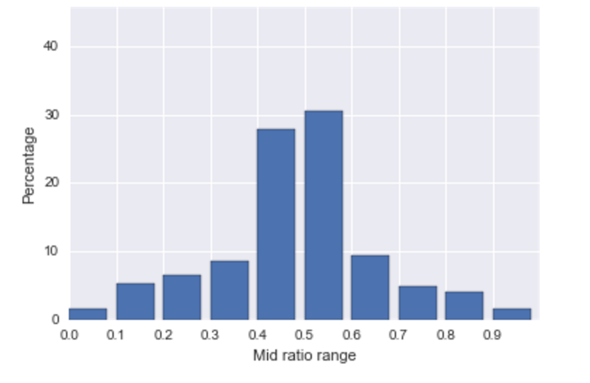
Distributions of the mid-ratios for colony triples from RTS

Distributions of the mid-ratios for colony triples from other investigators

Probability of mid ratio within [0.4, 0.6] with change of lambda