Indoor place categorization based on adaptive partitioning of texture histograms

Abstract

How can we localize ourselves within a building solely using visual information, i.e., when no data about prior location or movement are available? Here, we define place categorization as a set of three distinct image classification tasks for view matching, location matching, and room matching. We present a novel image descriptor built on texture statistics and dynamic image partitioning that can be used to solve all tested place classification tasks. We benchmark the descriptor by assessing performance of regularization on our own dataset as well as the established Indoor Environment under Changing conditionS dataset, which varies lighting condition, location, and viewing angle on photos taken within an office building. We show improvement on both the datasets against a number of baseline algorithms.

Main article text

INTRODUCTION

Humans possess the remarkable ability to reliably localize themselves in the world under a multitude of conditions: Indoors and outdoors, in unknown terrain, with reduced senses during different weather conditions, and even under cognitive load while processing other tasks. But how do we solve this problem? Answering this question will not only give crucial insight into mechanisms of spatial cognition in the human brain but may also be important for self-localization of mobile robots.

For humans, the dominant sensory information used for place recognition is vision [1]. However, the mechanisms that lead from visual input to knowledge of a place are poorly understood. What are the features we look at to determine where we are? Or to detach the question from its anthropological context: What are the features that best discriminate between places? Optimal features for this task would have to be specific for a certain place but invariant to different views within the location [2].

It is important to distinguish these requirements from the requirements for vision-based Simultaneous Localization and Mapping (SLAM; see Section 1.1 for a more detailed discussion). The features required there (tracking features) need to be stable across successive camera frames and recognizable from slightly different viewpoints, whereas the features suitable for vision-only place recognition have much stronger invariance requirements. For example, place features need to be matched across completely different views from a place, and they need to be stable over long periods of time with varying illumination conditions. Consequently, successfully matching place features is a much harder task than matching tracking features.

But what are suitable place features for this task? On larger scales, simple, global image statistics have been found to be discriminative between places. In particular, a global texture histogram descriptor has been shown to work for place classification tasks ranging from city-scale to world-scale localization [3]. For indoor localization [4], also use histograms over relatively simple orientation descriptors on the Indoor Environment under Changing conditionS (INDECS [5]) database.

However, these features are very generic, and confusion may arise if the same texture feature is found in multiple areas of an image, e.g., at the ceiling and on the floor. In this paper, we present an approach that circumvents this problem by partitioning the image according to texture occurrences.

Related work

The problem of one-shot vision-based place categorization has mostly been investigated on a larger scale level for urban locations, e.g., by [6–9] for discrimination within a city and [10] for discrimination between two cities. In these studies, authors usually rely on visual features useful for the recognition of house façades to enable the discrimination between locations. However, if and how the above results can be transferred to the problem of a room-level indoor place classification is not clear.

In localization tasks in robotics, this question is often overshadowed by the development of vision-based SLAM (see [11] and [12] for a review). In SLAM applications, an autonomous, mobile agent is placed into and moved through an environment with no prior information about its location or surroundings. The agent then simultaneously builds a map of its surrounding and places itself within this map.

Vision-based SLAM typically operates by tracking salient features between successive camera frames and deriving self-movement from shifts and deformations of these tracked features, which is sometimes also called visual odometry [13]. Typically, tracked features are simple image patches, which are determined as unique landmarks in an environment (e.g., [14]) to avoid confusion with other locations.

Indoor place categorization is sometimes assessed in the ‘lost robot’ (also called ‘kidnapped robot’)-problem [15], where a mobile robot is placed at a random position and needs to find its place in a previously recorded map. Typically, this is done based on map features over the course of several frames, e.g., by RATSLAM [16]. However, in this study, we try to solve the lost robot problem in a one-shot approach using visual data only. There are other studies which employ a holistic visual descriptor, e.g., by [17] using color histograms, [4] and [18] using image statistics and [19] using Scale-invariant feature transform (SIFT [20]) descriptors.

Textons are histograms over densely sampled cluster assignments on Gabor filter responses, which have been primarily developed for image segmentation [21]. Despite this, they have been shown to be surprisingly strong in scene classification [22] as well as in some outdoor self-localization tasks [3].

One problem with using texture histograms for high-level image classification tasks is that the same texture may be found in multiple regions of an image where they belong to completely different elements of a scene. A common approach is therefore to partition an image (as, for example, in Spatial Pyramids by Lazebnik et al. [23]) and handle individual image portions separately. This is a very crude approach as partitions do not necessarily coincide with contentual segments of an image.

Here, we will address this issue by partitioning images adapted to their contents.

Task definitions

Finding a suitable measurement for the quality of a localization descriptor is not trivial. In the context of robot tracking, measurements of deviation from the ground truth position are commonly used [11], but this does not make sense in one-shot place categorization problem where neither metric information nor connectivity between places is known.

We define indoor place categorization as a classification problem, where labeled images of a location are used as training data for a classifier. Performance is evaluated as percent correct PC, sometimes also called recall [24], on test images. With true positives of class i as tp_i and false negatives as fn_i:

(1) $$\text{PC}=\frac{{\displaystyle \sum _{i}t}{p}_i}{{\displaystyle \sum _{i}t}{p}_i+f{n}_i}$$

Chance level of this measure is simply c = 1/n, where n is the number of classes.

The definition of place categorization depends very much on the definition of a place, which may be interpreted as categorization of only different views from one specific location [2] or may be defined as broadly as counting all images of a whole city as one place that is being categorized against other cities [10].

To assess indoor place categorization, we define three different conditions on which feature descriptors will be tested.

Room classification means that given a number of training images from each room, a classifier needs to determine the room of a test image. The spatial distance between sample images of each room may be up to a few meters and all viewing angles may occur, as well as different lighting conditions.

Location classification means that each location is one class, and variations within the class include only viewing direction and lighting.

View classification means that sample images are taken from the same location and in the same viewing direction. The same objects will be visible in images of the same class and only variations in illumination and slight shifts might occur. This condition is not strictly place categorization since it regards different views from the same location as different places but serves as a sensible control condition here.

METHODS

Adaptive partitioning of texture histograms

The proposed descriptor is calculated in four steps:

1. All image pixels are assigned into texture clusters (Textons).

2. Textons are partitioned by their occurrence in different image regions.

3. Images are partitioned according to Texton partitioning.

4. Separate Texton histograms are calculated for each image partition.

Textons is a term coined by Julesz in 1981 for small image patches described by second-order statistics that play a role in human peripheral vision [25]. Textons have later been introduced for image segmentation and texture classification by Malik et al. [21].

In the implementation by Malik which is used here, a vector of Gabor filter responses is assigned to each pixel in an image (for details, see [21]). A set of n_T = 256 clusters is precomputed on a training dataset, and each pixel is assigned the cluster with the least square distance to its response vector.

We also use a generalization to colored Textons similar to the approach described by [26]. Image RGB values are transformed to the opponent color space as described in [27]:

(2) $$\left(\begin{array}{c}\widehat{E}\\ {\widehat{E}}_{\lambda }\\ {\widehat{E}}_{\lambda \lambda }\end{array}\right)=\left(\begin{array}{ccc}0.06& 0.63& 0.27\\ 0.30& 0.04& -0.35\\ 0.34& -0.60& 0.17\end{array}\right)·\left(\begin{array}{c}{R}_{x,y}\\ G_{x,y}\\ B_{x,y}\end{array}\right)$$

Filters are run on all output channels (i.e., luminance (Ê), blue-yellow (Ê_λ), and green-red (Ê_λλ) channel) separately, and the filter outputs are concatenated before the clustering step.

Texton partitioning. In the next step, we partition Textons into their typical occurrence in different vertical parts of an image, such as floor, ceiling, or central area.

Let c_x,y,i be the Texton assignment from the previous step for image position x,y on indexed image i. We then build histograms per row (y) counting how many times a Texton was assigned to a Texton cluster C_j in all unlabeled test images 1_X(x) is the indicator function which is 1 if x ∈ X and 0 otherwise.

(3) $$r_{j,y}={\displaystyle \sum _{x,i}{1}_{C_j}}(c_{x,y,i})$$

From this, we derive an average vertical position of occurrence ȳ_j for each Texton cluster:

(4) $${ȳ}_j=\frac{{\displaystyle \sum _{y}y}·r_{j,y}}{{\displaystyle \sum _y{r}_{j,y}}}$$

We sort the clusters by yȳ_j and split the sorted list into n partitions such that the total histograms counts are approximately equal in each partition. Let ${\widehat{y}}_{\widehat{j}}$ be the sorted list of yȳ_j and $\widehat{j}(j)$ the sorting indices, then the normalized cumulative sums of Texton counts along their vertical positioning are:

(5) $$R_{\widehat{j}}=\frac{{\displaystyle \sum _{\widehat{j}\prime =1}^{\widehat{j}}{\displaystyle \sum _y{r}_{\widehat{j}\prime ,y}}}}{{\displaystyle \sum _{y,j}{r}_{j,y}}}$$

$R_{\widehat{j}}$ ranges from 0 to 1. This range is split into n partitions, and Texton clusters C_j are assigned to a partition p based on their placement in R:

(6) $$p(C_j)=1+\text{floor}\left(n·R_{\widehat{j}(j)}\right)$$

Image partitioning. Depending on camera angles, field of view, and objects in the scene, different portions of each image may be taken up by ceiling, floor, and central areas. We therefore partition each image n according to the total amount of Textons T_i(P) from each partition P.

(7) $$T_i(P)={\displaystyle \sum _{x,y}{1}_P}(p(c_{x,y,i}))$$

The splits between partitions S_i (P) of an image i of height h are put at:

(8) $$S_i(P)=\text{round}\left(h·\frac{{\displaystyle \sum _{p=1}^P{T}_i}(p)}{{\displaystyle \sum _{p=1}^n{T}_i}(p)}\right)$$

Texton histograms. Texton histograms are calculated separately for each partition. Histograms are normalized by dividing them by the height of their respective sections. The resulting vectors are concatenated into one feature vector of length $n·n_T$.

Baseline feature vectors

For baseline performance, we also evaluate several established visual feature descriptors derived from the biologically inspired vision models.

Hierarchical MAX (HMax)-model is an object recognition model based on the neocognitron [28] and popularized by Serre et al. [29], which has been used to model neuron receptive field properties found in the ventral stream of the primate visual cortex by Hubel and Wiesel [30]. We use the Cortical Network Simulator (CNS) [31] implementation of HMax with parameter settings and dictionaries as chosen by Serre et al. [29]. Details of the implementation can be found in [29].

HMax features are included in this comparison because they have been shown to be able to discriminate well between object categories [29], which make them a good representative of landmark-based feature vectors. Based on the assumption that the presence or absence of object classes (like, for example, dishes in a kitchen, chairs in a conference room) are discriminative for places, HMax features might perform satisfactorily for self-localization as well.

Gist is a low-dimensional feature vector designed to capture the gist of a scene developed by Oliva et al. It consists of the first few principal components of spectral components on a very coarse grid (8 × 8) as well as on the whole image. Gist features are of special interest here because the algorithm has developed in for scene recognition task. For instance, Oliva et al. have found in [32] that Gist features successfully distinguish between scene categories like forest and city, and it has been hypothesized that humans use similar features for rapid scene classification tasks [33].

Since there is a strong relation between scenes and locations, Gist features are promising candidates for localization.

Spatial pyramids

Spatial pyramids have been introduced by Lazebnik et al. [23]. In this approach, histograms over low-level features in image regions of different size are calculated and concatenated to one large feature vector. The features used here are densely sampled SIFT [20] descriptors, and we test a three-level pyramid. For the sake of comparability, we omit the custom histogram matching support vector machine (SVM) kernel used by Lazebnik and use the same linear kernel and regression method also employed for other models.

Luminance histogram. As an additional control to test whether the task can be completed on very simple features, we also test a simple luminance histogram over the grayscale values of the image.

Room, place, and view categorization

To test how well potential place feature discriminates between rooms, places. and views, we evaluate performance as PC labels in one-versus-all classification, where all images taken from one room/place/view (see section on Task definitions) are samples of one class. Classification is performed as linear regression with leave-one-out cross-validation for parameters on the feature vector, which has been reduced to 128 components using principal component analysis (PCA) to ensure all descriptors have the same dimensionality. Each test is repeated 50 times with different random splits between test and training data to determine mean performance and mean error. All classifications are performed using the Grand Unied Regularized Least Squares (GURLS) classification package for MATLAB [34].

All source codes, datasets, and trained dictionaries required to reproduce the results of this study can be freely downloaded from http://www.informatik.uni-bremen.de/cog_neuroinf/indoorstudy. We also provide data on parameter tuning as applicable to the models in the supplemental materials.

Test datasets

INDECS database. The INDECS database by Pronobis et al. [5] is a collection of 3252 indoor photos taken from five different under three different lighting conditions (sunny, cloudy, and night). Photos are sorted by the position they are taken from, viewing angle and lighting condition (see Figure 1). We use subsets of the database sorted into different categories to test the different place categorization conditions:

Figure 1.

Example images from the INDECS database for cloudy (A), night (B), and sunny (C) condition.

For the room classification task, five rooms with 216 images per room are randomly selected. Ten images per class are used for training and the rest for testing. The place classification task picks 90 locations with 12 images per class, of which five are used for training and the rest for testing. The view classification task runs on 50 different views, where location and viewing angle are fixed, so only three samples per class are available. One sample is used for training and the rest for testing.

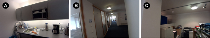
3Rooms. To ensure that our results are not specific to one dataset, we created an additional image dataset consisting of pictures taken from three connected rooms (see Figure 2). For the classification, we took 543 pictures at human eye level from different locations and different view directions from the three rooms.

Figure 2.

Example images from kitchen (A), hallway (B), and printer area (C).

RESULTS

INDECS classification

For the classification tasks on the INDECS database, there is a strong dependence of performance on task condition (see Figure 3). Although samples were taken from the same image dataset, feature vectors rank differently depending on how the classes are defined. Performance on luminance histogram is generally very low and near chance level for all three tasks.

Figure 3.

Classification performance of room, location, and view classification task in PC by feature vector. Dashed lines mark chance levels. APTH: Adaptive partitioning of texture histograms. APCTH: Adaptive partitioning of color texture histograms. SpPyr: Spatial Pyramids. LumHist: Luminance histogram. CTexton: Colored Textons.

Our proposed model (Adaptive partitioning of texture histograms, APTH) as well as the variant running on colored Textons (Adaptive partitioning of color texture histograms, APCTH) performs well on all three place categorization tasks. For room classification (Figure 3 left), we achieve 48.10 ± 0.53% correct on APCTH, which outperforms the colored texton approach of 46.34 ± 0.56% and lies well above all other control models. Both runs were performed with n = 2 partitions.

On location classification performance is much lower, which can be explained by the higher number of classes and also the higher confusion between locations within the same room. Adaptive partitioning again leads to stronger performance (APTH: 14.20 ± 0.32%, APCTH: 10.39 ± 0.29%) than classification on holistic Texton histograms (Texton: 11.88 ± 0.31%, Colored texton: 9.76 ± 0.31%). Interestingly, using color leads to higher performance on room classification but is derogatory for performance on location classification.

On view classification, all Texton-based approaches are outperformed by the control models that employ fixed image partitioning (Gist: 89.48 ± 0.49%, Spatial Pyramids: 84.36 ± 0.57%). However, adaptive partitioning of Textons still leads to a huge improvement over raw Texton histograms (APTH: 64.24 ± 0.76%, Texton: 42.56 ± 1.05%).

3Rooms classification

In the 3Rooms dataset, we test room categorization performance on a dataset that has fewer (3) but more diverse rooms, where a larger number of image samples per room is available. Performance results for the room classification task are shown in Figure 4. Again, room classification fails on the luminance histogram, for which performance remains at chance level. For a low sample count (Figure 4 left), APTH yields only a slight improvement over Textons (APTH: 56.62 ± 1.37%, Textons: 54.79 ± 1.69%), and both are outperformed by unpartitioned colored Textons (60.96 ± 2.00%).

Figure 4.

Classification performance of room classification task in PC by feature vector for different number of training samples. Dashed line marks chance level.

However, as more samples become available (Figure 4 right), APTH performance picks up leads to near perfect labeling (94.94 ± 0.36%), hinting that after partitioning, more task-relevant information is encoded in the descriptor.

DISCUSSION

We have shown that adaptive partitioning of texture histograms can provide a powerful image descriptor to perform several different place recognition tasks and find that our descriptor outperforms all tested baseline models in most of the tested place classification conditions.

The performance gain over vanilla global Texton histograms can be attributed to reduced confusion when the same Texton assignment appears in different areas of the image where they represent different contentual elements.

The rejection of both Gist and Spatial Pyramid features may be surprising, as they have both been introduced in a scene recognition context, which is often closely linked to place recognition. A possible explanation is that Gist has been tested on scenes downloaded by a keyword from photographic image databases [32]. However, when a photographer pictures a certain scene, there is often a default view that is taken which is specific to the scene at hand [35, 36]. For example, a tropical beach is commonly portrait with the vanishing point along the shore, the sun across the sea and a number of palm trees on the opposing side. Such artificial features may be caught by Gist, but they are not inherent to the location when photos are taken in random angles. A similar argument may be made for the Spatial Pyramid descriptor.

The poor performance on HMax descriptor may be attributed to the fact that the hierarchical HMax architecture picks on complex features that are unique to certain objects [32]. For example, in a kitchen, a typical HMax feature might be responsive to a pot or an oven. Since these are valuable tracking features, they lead to a strong performance in the view matching task. But individual, tracked objects would only be present in a limited number of views at the location and so they do not generalize well to other views from the same place.

Our results therefore highlight that place recognition is a task which is different from other tasks typically solved in pattern recognition problems such as object detection, scene categorization, or feature tracking between successive camera frames as found, e.g., in SLAM applications.

But why do Texton histograms in general and adaptively partitioned Texton histograms in particular generalize? The mechanisms are still poorly understood and should be a subject of future studies. However, one possible explanation is that Textons are designed to discriminate between surface textures and therefore attributes such as material types of the surrounding environment. Surface types are common to a more generic class of objects found at certain places than individual objects themselves. For example, the existence of metallic surfaces may be indicative of a kitchen because many metallic objects may be found there, and they are distributed across the whole room.

Therefore, we hypothesize that a suitable visual place descriptor should be geared at recognizing surface structure instead of objects.

Acknowledgments

This work was supported by DFG, SFB/TR8 Spatial Cognition, project A5-[ActionSpace].

References

1. , , , , . Spatial information content and reliability of hippocampal CA1 neurons: effects of visual input. Hippocampus. 1994;4(4):410–21. [Cross Ref]

2. , , , . From pattern recognition to place identification. In: , , , , , editors, Spatial cognition, international workshop on place-related knowledge acquisition research. Aachen (Germany): CEUR Workshop Proceedings; 2012. p. 39–44. http://ceur-ws.org/Vol-881/

3. , . Low-level global features for vision-based localization. In: , , , editors. Proceedings of the KI 2013 Workshop on Visual and Spatial Cognition, Koblenz, Germany, September 17. Aachen(Germany): CEUR Workshop Proceedings; 2013. p. 5–12. http://ceur-ws.org/Vol-1055/

4. , . A realistic benchmark for visual indoor place recognition. Rob Auton Syst. 2010;58(1):81–96. [Cross Ref]

5. , . A discriminative approach to robust visual place recognition. 2006 IEEE/RSJ International Conference on Intelligent Robots and Systems, 9–15 October, Beijing. Piscataway (NJ): IEEE; 2006. p. 3829–36.

6. , . An Image-based System for Urban Navigation. British Machine Vision Conference, 7–9th September, London, UK. Durham (UK): BMVA Press; 2004. p. 1–10.

7. , , . City-scale location recognition. IEEE Conference on Computer Vision and Pattern Recognition, 17–22 June, Minneapolis, MN, USA. Piscataway (NJ): IEEE; 2007.

8. , , . Avoiding confusing features in place recognition. In: Computer Vision - ECCV. 2010. p. 748–61.

9. , , . City-scale landmark identification on mobile devices. IEEE Conference on Computer Vision and Pattern Recognition, 20–25 June, Providence, RI. Piscataway (NJ): IEEE; 2011.

10. , , , , . What makes Paris look like Paris? ACM Transact Graph. 2012.

11. , . Simultaneous localization and mapping: part I. IEEE Rob Autom Mag. 2006;13(2):99–110. [Cross Ref]

12. , . Simultaneous localization and mapping (SLAM): part II. IEEE Rob Autom Mag. 2006;13(3):108–17. [Cross Ref]

13. , , . Visual odometry. Proceedings of the IEEE Computer Society Conference on Computer Vision and Pattern Recognition. 2004;1: 652–9.

14. , . Bearing only SLAM using colour-based feature tracking. Proceedings of the Australasian Conference on Robotics and Automation, Auckland. Brisbane (Australia): Australian Robotics and Automation Association Inc; 2002.

15. , . Quick and dirty localization for a lost robot. IEEE International Symposium on Computational Intelligence in Robotics and Automation, Monterey, CA, USA. Piscataway (NJ): IEEE; 1999. p. 262–7.

16. , , . Outdoor simultaneous localisation and mapping using RatSLAM. Field Serv Rob. 2006. p. 143–54. [Cross Ref]

17. , , . Visual topological mapping and localisation using colour histograms. Proceedings of the International Conference on Control, Automation, Robotics and Vision, 17–20 December, Hanoi, Vietnam. Piscataway (NJ): IEEE; 2008.

18. , , . Mobile robot self-localization based on global visual appearance features. Proceedingsof the IEEE International Conference on Robotics and Automation, 14–19 September, Taipei, Taiwan. Piscataway (NJ): IEEE; 2003. p. 1271–6.

19. , , . Global localization using distinctive visual features. IEEE/RSJ International Conference on Intelligent Robots and Systems, September 30–October 4, Lausanne, Switzerland. Piscataway (NJ): IEEE; 2002. p. 226–31.

20. Lowe D. Object recognition from local scale-invariant features. IEEE Seventh International Conference on Computer Vision, September 20–27, Kerkyra, Greece. Piscataway (NJ): IEEE; vol. 2. 1999. p. 1150–7.

21. , , , . Contour and texture analysis for image segmentation. Int J Comput Vision. 2001;43(1):7–27. [Cross Ref]

22. , . When is scene identification just texture recognition? Vision Res. 2004;44(19):2301–11. [Cross Ref]

23. , , . Beyond bags of features: spatial pyramid matching for recognizing natural scene categories. IEEE Computer Society Conference on Computer Vision and Pattern Recognition, 17–22 June, New York, NY, USA. Piscataway (NJ): IEEE; vol. 2. 2006, p. 2169–78.

24. , . A systematic analysis of performance measures for classification tasks. Inf Process Manage. 2009;45(4):427–37. [Cross Ref]

25. Julesz B. Textons, the elements of texture perception, and their interactions. Nature. 1981;290:91–7. [Cross Ref]

26. , . Color textons for texture recognition. British Machine Vision Conference, 4–7 September, Edinburgh, UK. Durham (UK): BMVA Press; 2006. p. 1099–108.

27. , , , . Color invariance. IEEE Trans Pattern Anal Mach Intell. 2001;23(12):1338–50. [Cross Ref]

28. Fukushima K. Neocognitron: a self-organizing neural network model for a mechanism of pattern recognition unaffected by shift in position. Biol Cybern. 1980;36(4):193–202. [Cross Ref]

29. , , . A feedforward architecture accounts for rapid categorization. Proc Natl Acad Sci. 2007;104(15):6424–9. [Cross Ref]

30. , . Receptive fields and functional architecture of monkey striate cortex. J Physiol. 1968;195:215–43.

31. , , . CNS: a GPU-based framework for simulating cortically-organized networks. Technical report. Cambridge, MA: Massachusetts Institute of Technology; 2010.

32. , , . Modeling the shape of the scene: a holistic representation of the spatial envelope. Int J Comput Vision. 2001;42(3):145–75. [Cross Ref]

33. , , . How long to get to the gist of real-world natural scenes? Visual Cognit. 2005;12(6):852–77. [Cross Ref]

34. , , , . GURLS: a toolbox for large scale multiclass learning. Big Learning Workshop at NIPS, 12–14 December, Granada, Spain. Red Hook (NY): Curran Associates; 2011. http://cbcl.mit.edu/gurls/

35. , , . Why is real-world visual object recognition hard? PLoS Comput Biol. 2008;4(1):e27. [Cross Ref]

36. , , , , , , , , , , , , . Dataset issues in object recognition. Heidelberg, Berlin: Springer; 2006.

Competing Interests

The author declares no competing interests.

Public Interest Statement

As humans, we possess the remarkable ability to be almost universally able to name what place we are currently at or at which place a picture might have been taken. Here, we show a novel method of how such one-shot place classification can be performed by a computer vision system.

Publishing Notes

© 2014. Sven Eberhardt. This work has been published open access under Creative Commons Attribution License CC BY 4.0, which permits unrestricted use, distribution, and reproduction in any medium, provided the original work is properly cited. Conditions, terms of use and publishing policy can be found at www.scienceopen.com.