Near-Earth Magnetotail Reconnection Powers Space Storms

Abstract

Space storms 1 are the dominant contributor to space weather. During storms, rearrangement of the solar wind’s and Earth’s magnetic field lines at the dayside enhances global plasma circulation in the magnetosphere 2,3 . As this circulation proceeds, energy is dissipated into heat in the ionosphere and near-Earth space. Because Earth’s dayside magnetic flux is eroded during this process, magnetotail reconnection must occur to replenish it. But whether dissipation is powered by magnetotail (nightside) reconnection, as in storms’ weaker but more commonplace relatives, substorms 4,5 , or by enhanced global plasma circulation driven by dayside reconnection is unknown. Here we show that magnetotail reconnection near geosynchronous orbit powered an intense storm. Near-Earth reconnection at geocentric distances ~6.6-10 Earth radii – likely driven by the enhanced solar wind dynamic pressure and southward magnetic field – is observed from multi-satellite data. In this region, magnetic reconnection was expected to be suppressed by Earth’s strong dipole field. Revealing the physical processes that power storms and the solar wind conditions responsible for them opens a new window into our understanding of space storms. It encourages future exploration of the storm-time equatorial near-Earth magnetotail to refine storm driver models and accelerate progress toward space weather prediction. The solar wind flow imparts energy to Earth’s magnetosphere that is dissipated as heat during substorms and storms. Substorms 4 are commonplace (several per day) cycles of solar wind energy capture and dissipation lasting 1 to 3 hours, occurring under moderate or active solar wind conditions. Initially stored as magnetic energy in Earth’s nightside magnetosphere, the magnetotail, this energy is abruptly released as particle energy by magnetotail reconnection, 20 to 30 Earth radii (RE) downtail 5 . Substorms, which produce continent-scale, bright auroras, do not have harmful space weather effects because they do not substantially affect the ring current (westward-drifting, tens of keV-energy ions, Fig. 1A) or the radiation belts (eastward-drifting relativistic, “killer” electrons, Fig. 1A), both of which encircle Earth near geostationary orbit (at geocentric distances R~6.6RE). Storms are infrequent (about one per month), last several hours to days, occur under active or very active solar wind conditions (peak or declining phase of the solar cycle), produce global-scale, most brilliant auroras and have severe space weather effects 2 , as they are associated with ion energization in the ring current 1 and electron acceleration in the radiation belts 6 . Magnetotail (nightside) reconnection also occurs during storms, but whether it can power them or is a mere byproduct of the global flux circulation driven by dayside reconnection is unclear: from 20-30 RE downtail, where nightside reconnection typically occurs, its outflows cannot reach inside geostationary orbit to energize the storm-time ring current and radiation belts 7 . Moreover, at such large downtail distances, the magnetic energy per particle in the lobes (Fig. 1B), Em =miVAL 2 =Blobe 2/μ0Ni, available for local particle heating (expected 8 to be: ΔTi ~13%Em ~3keV) is lower than typical storm-time ring current particle energies (Note: VAL: inflow Alfvén speed; Blobe: lobe magnetic field ~20nT; Ni: ion density, ~0.1/cm3; and mi: ion mass). If reconnection were to occur much closer to Earth (near geostationary orbit) it could be more geoeffective and powerful, but it is thought to be impossible there 9 due to the stabilizing effect of Earth’s strong dipole. Indeed, although on a few occasions reconnection has been suggested to take place at R<15RE, 10-11 it has been neither incontrovertibly identified nor placed energetically in the context of space storms. Thus, despite significant advances over the last ten years in our understanding of energy conversion during their weaker relatives, substorms, whether storms are powered by nightside reconnection or by the global circulation driven by dayside reconnection has been an open question since the dawn of the space age. Here we report the first comprehensive in-situ observations of magnetotail reconnection directly powering a storm from as close to Earth as ~8RE. 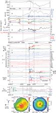From 03:00 to 06:00UT on 20 December 2015, during the main phase of an intense storm, the THEMIS P3, P4, P5, and GOES G13 satellites (Methods M1) were near the magnetic equator (Fig. 1A-B), well-situated to observe magnetotail reconnection. The solar wind’s large southward magnetic field, Bz,gsm<0 (Fig. 2A), and dynamic pressure, Pdyn (Fig. 2B), imparted sufficient energy to the magnetosphere to intensify the ring current and ionospheric heating (attested by ground-based indices in Extended Data Fig. 1A, 1B) to values typical during such storms 1,3-4 . Immediately following a dynamic pressure increase during the above time period, ground magnetic pulsations at ~04:46UT (Fig. 2B) signified intensification of magnetotail reconnection 12 . Around that time, all the abovementioned satellites observed a Bx-dominated (tail-like) field (Fig. 2E, 2F, 2I), a prerequisite for reconnection. In particular, because P5 and P3 or P4 observed Bx with opposite signs from 04:00 UT to 05:00 UT (Fig 2C), they bracketed the neutral sheet (where Bx = 0) and were close to it most of the time (as ∣Bx∣<Blobe). Thus, they were well positioned to observe the current sheet and its evolution, allowing us to compute (M6) its average density, Jy, (Fig. 2D). Peaking at ~80nA/m2, Jy became at least 10 times greater than during typical substorm pre-onset times 13 . The current sheet’s earthward-most extent is thus expected to be unusually close to Earth 14 , explaining why the field at G13’s geostationary location was also tail-like in both observations and empirical models 15,16 (Fig. 1A-B). All these conditions favor near-Earth reconnection. At ~04:46:40UT, G13’s Bz began to increase (Fig. 2E) toward Earth’s local dipole value (Bz,dipole~+111nT) as fluxes of high-energy (>100keV) particles intensified (Extended Data Fig. 1G-H). Simultaneously, P5 started to observe a bipolar Bz (Fig. 2F), southward-then-northward (negative-then-positive), correlated with fast, tailward-then-earthward Vx (negative-then-positive, Fig. 2G) and heating (Extended Data Fig. 1J). (Note that THEMIS plasma data were corrected for the presence of O+ , in M3, and energetic particles in M4.) Similar Bz and Vx signatures were observed at P4 (Fig. 2I-J), south of the neutral sheet, though the tailward flows at P4 were slower than at P5, likely because P4 was farther away from the neutral sheet than P5 at the time (Fig. 1C). We interpret these observations (Fig. 1B-C) as a reconnection region appearing between G13 and P4 (X=−6.1 to −9.5RE) at ~04:46:40UT and retreating tailward of P5 and P4 approximately 2min later, at ~04:48:30UT (marked as “X-line” in Fig. 2H-I). The nearly simultaneous initiation of opposing Bz excursions at G13 and P4 at ~04:46:40UT suggests that reconnection started midway between them, at X~ −8RE. The estimated tailward retreat speed ((−9.5)-(−8))RE/2min~ −75km/s) is similar to that in previous (substorm-time) reconnection observations farther from Earth 17 . During the fast flow period (Fig. 2G) when reconnection was locally active (Δt = 04:45-04:57UT, horizontal bar above Fig. 2A, C, E) the reconnection electric field ERX=Ey (Fig. 1C) at P5 was intermittent but consistently positive, comprising intense, ~1min-duration pulses (Fig. 2H: Ey,peak~100mV/m ~0.1VALBlobe, for Blobe~120nT, and Ni~0.1/cc, the measured lobe density). These bespeak of rapidly recurring, fast, impulsive reconnection. Multiple Bz<0 excursions at P5 (Fig. 2F) after the passage of the first X-line were embedded within persistently earthward flows (Vx>0, Fig. 2G). These could be secondary (weaker) X-lines swept by the outflow of the first (primary) X-line. We focus our attention on the 04:46:30 to 04:50:00 UT interval (vertical solid lines in Fig. 2E-J), which encompasses the primary X-line. We next establish that this nearly geostationary reconnection event has the hallmarks 18 of an active reconnection region: inflows; outflows threaded by Bz of the correct polarity; and a Hall system of electric fields, EHS, and currents, JHS, arising from separation of ions and electrons in the ion diffusion region and leading to a quadrupolar out-of-plane magnetic field, By (Fig. 1C). As the X-line retreats tailward, the satellites move earthward in the frame of the X-line (dashed lines in Fig. 1C). When cast in Bx-Bz space (Fig. 3), their observations can be compared to expectations from reconnection 18 , from either side of the X-line (Bz=0) and/or the neutral sheet (Bx=0), as measured in sequence by individual satellites, or even simultaneously by multiple satellites. We find that on both sides of the neutral sheet, the reconnection outflows (Vx) are directed away from the X-line and the inflows (Vz) are directed towards it (Fig. 3A, 3C, per Fig. 2G, 2J), as also corroborated by ion distribution functions (M5). The reconnection electric field (Ey, Fig. 3B; Extended Data Fig. 2B, 2D) is strongest and consistently positive across the entire reconnection region when ∣Bz∣ is large. The Hall electric field (E⊥,HS~Ez, Fig. 3D; Extended Data Fig. 2F), even more intense than Ey, points towards the neutral sheet from both sides of it. The parallel electric field (E∥, Fig. 3F; Extended Data Fig. 2H) observed clearly only at P5 (closest to the neutral sheet), reverses sign across the X-line. The magnitude and direction of E⊥,HS and E∥,HS in these observations agree with simulations 19 . A quadrupolar out-of-plane magnetic field, By, at P3, P4, P5 and G13 (Fig. 3E; Extended Data Fig. 2E) is also consistent with expectations 18 (By,HS, blue arrowheads/tails in Fig. 1C). The associated in-plane currents, JHS, approximated as Jx~(1/μ0)∂By/∂z from P3, P4, and P5 measurements (M7), flow away from the X-line at locations far from the neutral sheet (∣Bx∣>>0) and toward the X- line near it (Fig. 3G, consistent with black open arrows in Fig. 1C). The earthward field-aligned current is tens of nA/m2. If a fraction of it were to close through the ionosphere (with a mapping factor of >1000), it could provide several μA/m2, consistent with bright aurorae 19 . Comparing the solar wind flux input to the magnetosphere (M8) based on solar wind measurements, ΔtΦin ~0.2GWb, to the flux transport measured at THEMIS, Δt∫Eydt~0.053GWb/RE, provides an estimate of the magnetotail reconnection region’s effective width, ΔY~ ΔtΦin/Δt∫Eydt~ 4RE, which is considerably smaller than the magnetotail width (~40RE). Similarly, comparing the magnetospheric energy dissipation, ΔtUmd~ 0.82PJ, estimated from magnetospheric activity indices (M8), to the time-integrated Poynting flux into the magnetotail current sheet as observed at P5, Δt∫Szdt ~0.0228PJ/RE 2, provides an estimate of the effective reconnection area, ΔX·ΔY~ ΔtUmd/Δt∫Szdt~ 36RE 2~ 9·4RE 2 (the rectangle in Fig. 1A). The flows observed at THEMIS lasted only ~10min, even though the storm continued for hours. Multiple activations of tail reconnection at different azimuthal locations may have provided the aggregate energy conversion over the entire storm’s lifetime. The width, duration, intermittency, and flux/energy transport efficiency of storm-time reconnection outflows are similar to those of bursty bulk flows during substorms 21 . However, fast storm-time reconnection operating near geostationary altitude (where Blobe~120nT, six times that at 20-30RE) can be ~36 times more effective in energy conversion than during substorms (since Em∝Blobe 2) and have unimpeded access to cis-geostationary altitudes to efficiently power the storm-time ring current and radiation belts. What led to reconnection so close to Earth? The storm-time magnetic model TS0415, with input from the observed solar wind Pdyn and Bz,GSM (M9), exhibits intense, near-Earth (X~ −8RE) current sheet thinning and an equatorial Bz minimum (Fig. 1B; Extended Data Fig. 3). Consistent with our pre-reconnection observations at G13 and THEMIS (Fig. 2E, 2F, 2I; Extended Data Fig. 4), these conditions are conducive to magnetic reconnection. Since such intense solar wind driving is common during storms, it is likely that near-geostationary storm-time reconnection is also common, though elusive due to the extreme thinness of the current sheet (Fig 1C), the rarity of storms, and the scarcity of observations in this region. Studying these findings statistically and exploring the nature of energy conversion by retargeting current satellites or with future missions would be important for advancing our understanding of reconnection in many astrophysical and laboratory settings as well as for space weather modeling. Methods M1. Satellites and instrumentation The ARTEMIS 23 (P1, P2) high lunar orbiters located in the solar wind at the time of interest and the THEMIS 24 (P3, P4, P5) high Earth orbiters are identical satellites, also referred-to by their letter identifiers TH-B, -C, -D, -E, -A for P1-5, respectively. Data were accessed and processed using the Themis Data Analysis Software (TDAS), a plug-in of the Space Physics Data Analysis System 22 (SPEDAS) V3.0. Onboard Fluxgate Magnetometer 25 (FGM) and ground-processed Electric Field Instrument 26 (EFI) spin-fits (spin-period, Tspin, is 3-4 s depending on satellite) were used. For EFI ground processing, Fast Survey 27 voltages (at 8 samples/s) from the long sphere wires were utilized. Spurious spikes in these voltages due to shadowing by the satellite body were removed, then the voltages were spin-fit to produce the two spin plane E-field components. Spin-averaging of spin-axis voltages resulted in the third E-field component. Coordinates are discussed in the next section (M2). Ions and electrons between ~5 eV and ~30 keV were measured by the Electrostatic Analyzer 28-29 (ESA); those between ~35keV and ~1MeV were measured by the Solid State Telescope 24 (SST). Neither instrument provides ion mass discrimination. Standard calibration, background subtraction (photoelectrons, secondary electrons, internal scattering, and penetration), and satellite potential correction were implemented for the ESA 29 . Standard energy and efficiency corrections were performed for the SST. Energy spectra from the ESA and SST merged into combined distributions were used to compute moments and particle spectra. The moments were then corrected for the presence of oxygen (M3). The presence of significant fluxes of relativistic electrons caused SST fluxes to be saturated (M4) after 05:16UT, but that has no effect on the conclusions of our study, which is focused on 04:40-05:00 UT (Fig 2; Extended Data Fig. 1). Distribution function cuts discussed in a separate section (M5) are from ESA alone. Data from the GOES 13 (G13) satellite are from the magnetometer 30 , medium-energy proton and electron, and high-energy proton and electron instruments 31 . Magnetometer data, obtained from the National Geophysical Data Center (NGDC), are at 0.513s resolution. Protons between 95 and 575 keV are at 16.4 s resolution, and those at 2.5 MeV are at 32.7 s resolution. Electrons 40 – 475 keV are at 60 s resolution; those at 0.6 and 2 MeV are at 4.1 s resolution. Only the 40-475 keV electrons were obtained as omni-directional, calibrated quantities; all others were retrieved as uncorrected, directional fluxes and were averaged and rescaled to match levels published online. Although absolute fluxes are only approximate (within a factor of 2), relative flux changes, as used in this paper, are reliable. The Auroral Electrojet (AE) Index 32 from the Kyoto World Data Center 2 (WDC2), at 1min resolution is also used. It denotes the strength of ionospheric circulation, substorm activity, Joule heating and ionospheric dissipation 4 . The OMNI Database was used to retrieve the Disturbance Storm-Time (Dst) Index 32 (a measure of the total ring-current energy), at the same time resolution as from WDC2. The Dst’s time rate of decrease is a measure of storm-time solar wind energy conversion and deposition (dissipation) into the ring current. However, the raw index also responds to magnetopause currents, which are unrelated to the ring current 33 . This effect can be corrected using the solar wind dynamic pressure. The pressure-corrected Dst, denoted Dst*, was used (M8) to compute the total magnetospheric energy dissipation 4 . Finally, we use data from the local horizontal, magnetic north component of the fluxgate magnetometer at Bay Mills, MI (bmls) 34,35 , at 0.5s resolution. M2. Coordinates Geocentric solar magnetospheric (GSM) coordinates 36 were used for solar wind data (X: sunward; Y: cross-product of Earth’s magnetic dipole axis and X; Z: completes the right-hand, orthogonal coordinate system). For nominal (non-storm) conditions, the GSM system is also used in the magnetotail, as it adequately describes the tail’s field line stretching and alignment with the Sun-Earth line (along XGSM) far from Earth’s dipole 37 . Under the storm-time conditions of our event, however, the model 15 field-line planes at THEMIS, as seen in Fig. 1A, were evidently rotated clockwise about ZGSM towards the magnetic meridian; measurements also exhibit this behavior. An appropriate system that is coplanar with the field lines prior to the onset of reconnection was therefore used. Clockwise rotation by a common ϕrot ~10° angle about the ZGSM axis at all satellites was found to minimize the absolute value of the By component during the undisturbed time interval, 04:30-04:40UT, at P5 and P3 (the two satellites straddling the current sheet but farthest from it at that time); this rotation is also consistent with the model field-line planes (Fig. 1A). We formally defined ϕrot as the angle between XGSM and the reverse of the instantaneous, time dependent, average position of the THEMIS satellites (their geometric center), -R GC, minus 10°. This allows us to analyze the reconnection phenomena in a natural coordinate system defined by the plane of the field lines. We rotated all vector THEMIS data (flows, fields, currents, distribution functions) accordingly. We refer to this rotated-GSM system as XYZ throughout this paper and reserve the notation XYZGSM for the pristine GSM coordinate system. Closer to Earth (at and inside geostationary orbit), another system, the solar magnetospheric (SM) system, in which the ZSM axis is exactly aligned with Earth’s magnetic dipole 36 , is used under nominal (non-storm) conditions, because a dipole is a reasonable approximation of Earth’s field. In our storm-time event, however, the near-geostationary model 15 field lines at G13 are distorted considerably from dipolar (Fig. 1B): they are stretched into a tail-like geometry by enhanced cross-tail currents. Hence, the SM system is not useful to show the G13 data, but the GSM system is, so we use it instead. Additionally, because G13 is near midnight (Fig. 1A), where meridional planes are expected to be parallel to the XZGSM plane, no further rotation about ZGSM is needed to match field-line planes. Indeed, when plotted in GSM, the G13 data (Fig. 2E, Extended Data Fig. 1F) show a dominant Bx component increase (indicating current sheet thinning) just prior to the interval of interest, Δt. No significant (out of plane) By was seen until near or just after reconnection onset, again indicating that the field line planes as inferred from the data are also approximately parallel to XZGSM. In summary, we use GSM coordinates everywhere in this paper except for THEMIS, where we use the rotated-GSM system rotated clockwise by ~10° about the ZGSM-axis to account for the rotation of the field-line planes. M3. O+ density fraction and associated plasma moment corrections The measured total ion and electron densities differ consistently from each other on all satellites (with Ni/Ne ~ 1/1.53), suggesting the presence of species heavier than protons. This is because the ESA and SST ion instruments directly measure the ion differential number flux at a given ion energy. Onboard software assumes that this flux is made up of protons only. When a heavier ion species is present, its true velocity is lower than derived by this instrument from the protons-only assumption at each measured energy. The velocity moment is thus overestimated by the square root of the heavier ion- to-proton mass ratio, resulting in a proportional underestimation of the ion density 38 . During storms, the oxygen fraction f=NO+/Ne in the plasma sheet and the ring current can be significant 39,40 . Assuming that O+ is the only species of significance other than protons, the measured density 38 is: Ni/Ne = 1 − f + f/(mO+/mp)½. For the average observed ratio at P5 (similar to that at P4), Ni/Ne ~ 1/1.53, we obtain f=0.46~0.5. Using this, we corrected the ion velocity and the pressure tensor (both scaled upwards). Temperature and magnetic energy per particle are unaffected by the presence of different species. Based on these densities, the relevant species inertial lengths are: dO+~911km, dp+~228km, and de−~5km. M4. SST saturation and background removal at P5 Prior to 05:16UT, fluxes of >35keV ions were below threshold, whereas fluxes of >35keV electrons were not significant enough to affect the electron moments. In the 04:48-04:50UT interval (around the time of X-line passage), increased background from >1MeV electrons moving through the instrument walls (evident in both ESA and SST spectra), was removed prior to moment computations by standard processing 29 , so it does not affect our study. After 15:16UT the 35-300 keV electron fluxes increased considerably. SST electron count rates exceeded 10ksamples/s. At these rates, background removal and dead-time corrections cannot reconstruct the true fluxes, which are then regarded as a lower estimate (saturated). However, ESA data are not saturated – standard ESA background removal results in good quality lower-order moments (velocity, density) because those are less dependent on energies measured by the SST. As a result of SST saturation after 05:16UT, higher-order moments (electron/ion pressure and temperature) are underestimated (e.g., over the double arrow in Extended Data Fig. 1J) and should be considered lower limits during that period. M5. Ion distribution functions A representative ion outflow distribution at P5, tailward of the X-line at 04:47:29UT (Extended Data Fig. 1L) and taken near the peak of the tailward flow period (Fig. 2G), demonstrates that the plasma sheet velocity moments contain two distinct populations: a warm, dense, predominantly equatorward-moving beam (phase space density peaking at Vz,gsm~ − 500km/s) and a hotter, tenuous, predominantly tailward-moving beam (peaking at Vx,gsm ~ − 1500km/s), typical of reconnection outflows 41 . Embedded in a hot plasma sheet of lower density (green contours enveloping the two beams in Extended Data Fig. 1L), these were moving equatorward at approximately the same speed as the other two components. This is consistent with plasma sheet reconnection, in which inflows and outflows (the first two components) are immersed in the ambient plasma sheet plasma (the third component). P4, farther from the neutral sheet than P5, based on its higher ∣Bx∣ value (Fig. 2C), did not observe a strong tailward outflow but an inflow (Vz>0) into the reconnection region (Fig. 2J). A representative ion distribution at P4 (Extended Data Fig. 1M) shows two cold equatorward-flowing beams (flowing approximately perpendicular to the magnetic field) separated by a factor of four in velocity (400km/s versus 100km/s) embedded in a third, hot isotropic population, likely ambient plasma sheet ions as seen at P5. The two cold beams are consistent with THEMIS’s total-ion instrument response to two cold O+ and H+ populations, both ExB drifting at the same speed, ~100km/s. Such a response is expected from the velocity transformation of energy bins into velocity bins, under the incorrect assumption that all ions at a given energy are protons (M3); it has been used in past studies for species discrimination on THEMIS 42 and other missions 43 . Also streaming parallel to the magnetic field (tailward), these beams are likely of ionospheric origin. Projection of the total flow (perpendicular inflow and parallel streaming) in the XGSM direction results in the tailward net flow (first moment of the distribution) observed at this time. Although the third hot ambient plasma sheet ion population is likely also a mixture of H+ and O+, it cannot be separated into its constituent species because its velocity is too small compared to its thermal velocity. M6. Cross-tail current density (Jy), position, and thickness estimation The average cross-tail sheet-like current (∂/∂z >> ∂/∂y, ∂/∂x=0) is approximately Jy=μ0 −1(∂Bx/∂z - ∂Bz/∂x) ~ μ0 −1∂Bx/∂z. Applying the commonly used Harris model 44 , Bx(Z)/Blobe=tanh(Z-ZNS/LCS) yields: Jy(Z)= (μ0LCS)−1 Blobecosh−2(Z-ZNS/LCS), where ZNS is the neutral sheet location and LCS the current sheet half-thickness. With Bx measured at two satellites and Blobe estimated from the plasma and magnetic field data (Fig. 2C), we can solve for the two unknowns, ZNS and LCS, and an estimate of the peak current, Jy(ZNS)=μ0 −1Blobe/LCS. Of the two adjacent satellite pairs (P5-P4, P4-P3), the one that straddled the neutral sheet typically produced the strongest current density estimate (Fig. 2D) and was used to obtain the current sheet parameters ZNS, LCS (Extended Data Fig. 1K). We also estimated Jy,GSM=μ0 −1(∂Bx,GSM/∂z,GSM - ∂Bz, GSM/∂x,GSM) directly from the magnetic field measurements on P3, P4 and P5 (without any other approximations), because those satellites are located approximately on the XZ-GSM plane (their YGSM average separation from their barycenter was only ~300km, whereas their XGSM and ZGSM average separations were 2500km and 2900km, respectively). Outside 04:25-05:15UT, when the current sheet was thicker than the inter-satellite separation, we obtained values that are nearly identical to those from the Harris model. Inside that time interval, the Harris model provided a larger current density estimate. This is understandable given that the Harris model solution is: (i) a fit to an equation, not an average, and (ii) obtained from 2 satellites at a smaller separation (δZ54~3300km, δZ43~3000km) than the 3-satellite linear dimension (δZ53~6300km), and thus able to better resolve a current sheet of scale LCS⪅δZ54 (Extended Data Fig. 1K) than the 3-satellite method. M7. Hall system current density, JHS, estimation The Hall system current for a thin sheet-like current (∂/∂z >> ∂/∂y, ∂/∂x ~ 0), JHS~Jx~ −μ0 −1∂By/∂z, comprises three current layers centered at the neutral plane: the middle one near the equator and the north and south ones on either side of the equator (Fig. 1C, black open arrows). The equatorial layer current sheets are expected to flow towards the reconnection site (across the magnetic field), whereas the off-equatorial layer current sheets are expected to flow away from the reconnection site (nearly along the field). We used the By measurements and inter-satellite Z-distance of the satellite pair that straddled the neutral sheet (Extended Data Fig. 1K) to compute the equatorial J HS currents. We estimated the off-equatorial J HS currents by assuming that the peak values of By were located halfway between the peak and the minimum of the cross-tail current (i.e., between the current sheet center and the current sheet boundary), LCS/2 away from the neutral sheet. If both paired satellites were located farther than LCS/2 (the presumed By peak) from the neutral sheet, δBy/δz was derived directly from the satellite By differences. If a pair straddled the anticipated By peak, then the By average, <By>, was taken as a proxy of the peak; the lobe By was assumed to be zero; and the spatial derivative was approximated as <By>/(LCS/2). These assumptions resulted in a continuous estimate of the three current sheet profiles thanks to the persistent Hall current system By signatures and the continuous proximity of the satellites to the current sheet. M8. Reconnection’s contribution to global flux and energy transport Here we assess the reasonableness of the reconnection region’s size estimated from the global-to-local flux and energy transport ratios integrated over the Δt~12min interval (04:45-04:57UT) when reconnection was observed to be active at THEMIS. The magnetospheric magnetic cumulative flux input is the solar wind electric field, Ey,sw ~VtotBz,GSM (Extended Data Fig. 1C-D), applied across a nominal, 40RE cross section of the tail at a 20% reconnection efficiency 45,46,21 , then time-integrated: Φin= 0.2·40RE·∫Ey,swdt (Extended Data Fig. 1E). Φin’s slope (~1GWb/hr) multiplied by Δt gives ΔtΦin~0.2GWb. The time-integrated flux transport per unit Y-distance in the magnetotail at P5 is: Δt∫Eydt =<Ey>Δt ~11.5mV/m·12min ~0.053GWb/RE (<Ey> is the average Ey from Fig. 2H over Δt). The ratio ΔtΦin/Δt∫Eydt provides an estimate of the tail reconnection region’s effective width, ΔY~4RE. We call it effective because reconnection is impulsive and likely localized; hence, it does not comprise a single X-line all across the active region. This effective width is considerably smaller than the tail width (~40RE). Thus, although intermittent and impulsive, the fast reconnection observed was effective in producing the requisite storm-time flux transport, even if only operating over a fraction of the tail width. The solar wind energy input rate to the magnetosphere 4,1,46,21 is: ε[W]= (4π/μ0)VB2sin4(θ/2)·lo 2, otherwise known as the Akasofu “epsilon” parameter, with θ= acos(Bz,GSM/Byz,GSM), lo =7RE. Its cumulative integral is: Uin= ∫εdt ~ 6.7PJ per hour (Extended Data Fig. 1E). Uin compares well (better than a factor of 2) with the cumulative integral of the magnetospheric energy dissipation (also in Extended Data Fig. 1E) computed from indices 4,1,46,21 , as: Umd=∫[4·1013(∂(−Dst*)/∂t + (−Dst*)/τR)+300·AE]dt ~ 4.1PJ per hour, where τR=1hr is the ring-current decay rate of O+ through charge exchange (for AE and Dst* see M1). We see that the magnetospheric energy dissipation during Δt is: ΔtUmd~0.82PJ. The time-integrated Poynting flux, Sz=(ExBy-EyBx)/μ0, into the current sheet at P5 (using data from Fig. 2F, 2H) is: Δt∫Szdt=Δt∫[(ExBy-EyBx)/μ0]dt=<Sz>Δt ~0.78mW/m2·12min ~0.0228PJ/RE 2 (<Sz> is the 12min average of Sz). The ratio ΔtUmd/Δt∫Szdt provides an estimate of the effective reconnection area, ΔXΔY= (0.82PJ)/(0.0228PJ/RE 2) ~36RE 2. Having already estimated ΔY~4RE, we obtain ΔX ~9RE, approximately ±30dO+ (or ±130dp+, also reasonable), based on reconnection exhaust size estimates from simulations and observations 18 . If centered at P5 when Vx, Bz reversed sign, the reconnection exhaust extends from just earthward of G13 to ~X=−15 RE (the rectangle in Fig. 1A-B). This is consistent with G13 observations of a strong Hall By. M9. Equatorial Bz minimum: model versus data The equatorial dipole field at P4 (Bz,dip~+28nT) alone is too large (compared to the lobe field) to allow tail reconnection so close to Earth. It is suppressed, however, by the Bz<0 contribution from the fringe field of the cross-tail current, which is particularly strong during storms. The cross-tail current strength is regulated by Pdyn as well as the amount of flux in the lobes (which is, in turn, controlled by the solar wind southward magnetic field, Bz,GSM). Both Pdyn and negative Bz,GSM are known to be enhanced during coronal mass ejections and stream-stream interaction regions 1 , the two main solar wind structure types leading to intense space storms. Therefore, reduced near-Earth magnetotail equatorial Bz, may be a commonplace occurrence under storm conditions. It is instructive to further examine evidence in our event that an enhanced Pdyn and negative Bz,GSM resulted in favorable conditions for near-geostationary reconnection. Storm-time models of the magnetosphere, such as the TS0415 model (see field lines drawn from it in Fig. 1A-B), parameterize current systems based on ensemble averages of in-situ magnetic measurements. Because of the extreme thinning of the current sheet during active times, such measurements are biased towards the plasma sheet boundary layer, where field lines flare out of the neutral plane. The resultant models exaggerate the negative Bz tail current contribution to the equatorial Bz profiles. Such models can, however, provide useful estimates of the location of a local minimum in the equatorial Bz, which is controlled by the equatorial distribution of the cross-tail currents. Examination of the equatorial Bz profile in TS04 (Extended Data Fig. 3) for the solar wind conditions just prior to reconnection onset in our event shows such a pronounced minimum (−10 nT to −30 nT) across the tail at XGSM ~ −7.5 to −8.5 RE. Such Bz values are, of course, unphysical: first, because reconnection should have occurred before they were attained, and second, because even if they materialize after reconnection, they are dynamically unstable due to JxB forces that will expel the resultant magnetic loop on the tailward side further tailward, out to the solar wind. Such negative Bz equatorial distributions, however, pinpoint the loci of anticipated equatorial Bz minima, dictated by a cross-tail current distribution consistent with the magnetospheric currents globally prescribed by the solar wind conditions at the time. In our event, they show that reconnection was likely to occur anywhere across the equatorial magnetotail (in Y) and near the X-distance where we observed reconnection onset, i.e., midway between G13 and P3-5, at XGSM~ −8RE. We next examine the observed magnetotail Bz just prior to reconnection onset (around 04:45:00-04:46:12UT), when LCS was less than the THEMIS inter-satellite separation (Extended Data Fig. 1K). All satellites were farther from the neutral sheet than LCS, as also evidenced by their large ∣Bx∣ (Fig. 2C, Fig. 2F, 2I). Because the Bz reduction was partly due to field-line flaring, some modeling is needed to determine the equatorial Bz. We use the simplest linear model of Bz’s falloff with distance from the equator (Extended Data Fig. 4). We infer an equatorial field that was small (0.54±0.01nT, <1% of Blobe) though still positive at the THEMIS satellites’ geometric center (XGSM~ −9.8RE). Such a Bz field is indeed small enough to overcome the stabilizing effect of electron magnetization and permit reconnection under external forcing 47 . Even lower values of equatorial Bz may have been realized closer to Earth, at the mid-point between G13 and P3, P4 and P5, resulting in yet another, spontaneous onset, path to the tearing instability 48 . Regardless of the specific kinetic process that may have caused current sheet tearing and reconnection onset (important in its own right), the overarching condition that led to the development of this Bz minimum is the solar wind driver -- in particular its strong Pdyn and negative Bz,GSM. The equatorial Bz inferred is already so low that small fluctuations in dynamic pressure could cause it to reconnect on timescales faster than spontaneous tearing-mode growth rates 49,50 . Extended Data Extended Data Fig. 1. Extended overview of reconnection region observations. (A) Dst index encompassing several days around the event. (B) AE index (black, left axis scale) and ground magnetometer magnetic pulsations from Bay Mills (bmls), band-pass filtered at 10s-120s (northward component δBX shown, in blue, in the right vertical axis scale; repeated from Fig. 2B for referencing the time of reconnection enhancement around the time of enhancement in pulsation amplitude). (C) Solar wind magnetic field at ARTEMIS P1 in GSM coordinates. In this and all subsequent panels showing vector quantities, black, blue, green and red traces correspond to the vector magnitude, and its X, Y, and Z components, respectively. Note that when not explicitly defined, X,Y, Z components refer to the GSM coordinate system rotated about the ZGSM axis by ~10° to account for the approximate rotation of the field-line planes on THEMIS at that time (M2). (D) Solar wind dynamic pressure, Pdyn (black); density, Ni (blue); velocity magnitude, Vtot (red) also at ARTEMIS P1, showing that the Pdyn increase was due to the Ni increase. (E) Cumulative integrals (M8) of: i) solar wind energy coupling function ε, Uin= ∫εdt (black); ii) flux input rate in the magnetotail by the solar wind electric field Ey,sw, Φin=0.2·40RE·∫Ey,swdt; and iii) magnetospheric energy dissipation rate computed from Dst and AE, Umd (blue).(F) G13 magnetic field components in GSM coordinates; (G) G13 proton fluxes at energies tabulated on the right (increasing flux corresponds to decreasing energy); vertical blue arrows show times of energization; (H) G13 electron fluxes corresponding to the energies tabulated to the right as in (G); vertical red arrows show times of energization; (I) P5 magnetic field components (shown for reference) in X, Y, Z rotated GSM coordinates; (J) ion (Ti) and electron (Te) temperatures at P5 (saturation noted after 05:16UT causes temperatures to be underestimated, but does not affect our conclusions (M4)); vertical blue and red arrows correspond to ion and electron heating, respectively. (K) Estimate of ZGSM location of the neutral sheet, ZNS (middle solid line), and current sheet thickness, LCS (represented by distances of the upper and lower solid lines from the middle one), obtained from Harris sheet model (M6), overplotted along with P3-P5 positions (colored dashed lines); vertical lines are same as in Fig. 2E-J; they correspond to the interval of interest (04:46:30 to 04:50:00UT) encompassing the fast flows (solid lines) and time of the X-line passage (04:48:30UT) by P5 and P4 (dashed line). (L) Representative ion velocity distribution function X-Z plane cut (X is positive to the left) during one spin near the peak tailward reconnection outflows at P5, showing simultaneous reconnection inflows from above the neutral sheet (M5). (M) Same as 1L but at P4, at approximately the same time, showing reconnection inflows from below the neutral sheet (M5). Extended Data Fig. 2. Correlation of flows, fields, and currents with Bx, Bz. Quantities plotted compactly in Fig. 3 are shown here in raw format, plotted against Bx, or Bz separately to reveal their correlation with these quantities, signifying adherence to expectations from the reconnection paradigm and revealing the full excursion of these quantities, which is obscure in color in Fig. 3. Quantities and units are listed in horizontal axes; Bx or Bz are listed in vertical axes (common for left and right panels). Different symbols correspond to various satellites in A-F and H and to different distances from the neutral sheet in G (as denoted in inserts). Colors, also representing satellites (P5/P4/P3 are magenta/blue/turquoise, respectively) in A-D and F further help differentiate the sources of data. Colors represent sign of Bz (red, blue for Bz<0, >0 respectively) in E, G and H. The time-interval plotted is 04:46:30-04:50:00UT (vertical solid lines in Fig. 2) except for some deviations for Vz, By, and Ez (denoted in the individual panels C, E and F), justified as follows: for Vz (restricted to 04:46:30-04:48:30UT, tailward of the X-line), the earthward side of the plasma sheet expanded lobeward, and the equatorward inflow (Vz) cannot be cleanly separated from outward expansion; for By (at G13 only, restricted to 04:46:30-04:47:45UT), the neutral sheet flapped southward (Extended Data Fig. 1K). and G13 moved closer to the neutral sheet as its ∣Bx∣ was suddenly reduced (Fig. 2E) and all its components became very noisy, presumably as it was immersed in the hot outflows from reconnection – beyond 04:48:30UT the reconnection exhaust moved quickly away from G13 as the X-line moved tailward; and for Ez (extended to 04:46:30-04:57:30UT) the interval is justified by the persistence of the Hall system electric field at P5-3 over the entire interval Δt (subsequent, secondary X-lines result in similar polarity Hall electric field, towards the neutral sheet from both sides). To reduce clutter from random fluctuations, low magnitudes of some quantities have been eliminated for Vx, By, Ez, and E∥, as listed in the respective panels (A, E, F and H). Extended Data Fig. 3. Model equatorial Bz. Equatorial Bz profile (color) from the TS04 model15 based on solar wind and Dst values at 04:45UT, with field lines (solid lines: above magnetic equator; dashed: below) and satellite locations from Fig. 1 superimposed (for reference). The magnetic equator in the model was determined as the surface of B r = B ⋅ r ^ reversals, as a function of Z. At the equatorial (X, Y) projections of THEMIS satellites, the model Bz ranges from −2.5 to −7nT. Extended Data Fig. 4. Equatorial Bz at THEMIS. Equatorial Bz at THEMIS. Linear fit to Bz data from THEMIS P5-3 immediately prior to reconnection onset, 04:45:00 – 04:46:12 UT, as a function of their distance DNS from the neutral sheet position, ZNS. The Harris sheet44 model was used to determine ZNS (M6). The inferred equatorial Bz is ~ +0.54nT.