1. INTRODUCTION
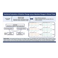
In clinical trials, primary study endpoints are often analyzed to determine whether the intended studies will achieve the study objectives with the desired statistical power. In practice, investigators can consider four different types of primary endpoints or outcomes according to a single study objective: (i) absolute change (i.e., the endpoint’s absolute change from baseline), (ii) relative change (e.g., the endpoint’s percentage change from baseline), (iii) responder analysis based on absolute change (i.e., an individual participant is defined as a responder if the absolute change in the primary endpoint exceeds a pre-specified threshold known as a clinically meaningful improvement), or (iv) responder analysis based on relative change. Although analyses based on these endpoints all appear reasonable, the following statements are often of great concern to principal investigators [1]. First, a clinically meaningful difference in one endpoint does not directly translate to a clinically meaningful difference in another endpoint. Second, these derived endpoints generally have different sample-size requirements. Third, and most importantly, these derived endpoints may not yield the same statistical conclusion (based on the same data set). Consequently, determining which type of primary endpoint is most appropriate and can best inform on disease status and treatment effects is of particular interest.
Some researchers have criticized responder analysis because of a loss of information; i.e., the statistical power of a trial decreases if a continuous outcome is categorized into a binary variable [2, 3]. Although responder analysis may come at the expense of power, it still provides value. For example, the original scale (continuous) outcome is used to make binary decisions, such as whether a patient should be hospitalized. In a heterogeneous disease, a subset of patients may have more benefit than others, thus resulting in a non-normal distribution of the outcome [4]. If the trial is aimed at investigating an additional second agent, and the proportion of patients with more benefit is of interest, responder analysis is more suitable [4]. Because of its benefits and drawbacks, [3] have suggested that responder analysis be used as a secondary analysis to better interpret findings from the main analysis. However, analysis using absolute change as an endpoint and the corresponding responder analysis have different statistical properties. Hence, investigating their differences in terms of statistical power, sample size, and conclusions is highly important.
To study the relative performance of these derived endpoints, in addition to mathematical derivations, we conducted a numerical study and real case study based on data on a recent rehabilitation program in lung transplant candidates and recipients [5]. The 6-minute walk distance (6MWD), a commonly used clinical indicator for patients with pulmonary disease, can be used as not only a prognostic factor but also as a health outcome variable [6]. For example, the 6MWD has been used to measure the functional status and exercise capacity of lung transplant candidates or recipients [7, 8]. Some studies have used the endpoint of the change in 6MWD from baseline (absolute change) as the outcome variable to evaluate the performance of pulmonary disease treatment [9], whereas others have performed responder analysis using 6MWD [10, 11]. Individuals can be defined as responders if they meet a pre-specified threshold of improvement in 6MWD and as non-responders otherwise. In one example, [11] have classified patient performance after rehabilitation according to the following criteria: good, 6MWD increase ≥50 m; moderate, ≥25 to <50 m; and non-response, <25 m. However, in another study [12], have reported that the minimum important change in 6MWD in chronic respiratory disease is 25 to 33 m. [13] have used 25 m as the threshold for equivalence in the change in 6MWD. Although the wider range of 6MWD is generally accepted as 25 to 30 m, the exact threshold of change in 6MWD that is clinically meaningful is under debate.
In this case study, for simplicity, we focused on statistical evaluation of a rehabilitation program in lung transplant candidates and recipients in terms of absolute change in 6MWD and responder analysis based on a pre-specified threshold (improvement) of 6MWD on the basis of absolute change. A comparison between the absolute change and responder analysis with various pre-specified thresholds was performed in terms of sample-size requirement and statistical power. In the next section, we presented statistical methods for analysis using absolute change as the study endpoint as well as the corresponding responder analysis. Additionally, we compared the performance of these study endpoints in terms of statistical power, sample size and study results/conclusions. In Section 3, we discussed a numerical analysis of the comparison between absolute change and responder analysis and a case study of a rehabilitation program in lung transplant candidates and recipients. Brief concluding remarks and recommendations were given in the last section of this article.
2. METHODS
2.1 Hypothesis testing for efficacy
Non-inferiority testing is commonly considered in randomized clinical trials evaluating the performance of a new drug or new treatment versus an active control (e.g., standard of care). The success of a non-inferiority trial depends on the selection of the study endpoint and the non-inferiority margin. As indicated earlier, for a given study endpoint, four types of primary endpoints exist: absolute change (e.g., endpoint change from baseline), relative change (e.g., endpoint percentage change from baseline), responder analysis based on a pre-specified improvement (threshold) in absolute change, and responder analysis based on a pre-specified improvement (threshold) in relative change. Consequently, the inference from responder analysis is very sensitive to the pre-specified threshold (cutoff) value [14]. For simplicity and illustration purposes, we examine the performance of the first two primary endpoints: absolute change and a corresponding responder analysis.
We assume a two-arm parallel randomized clinical trial comparing a test treatment (T) and an active control (C) with a 1:1 treatment allocation ratio. Let W 1 ij and W 2 ij be the original response of the ith patient in the jth treatment group at baseline and post-treatment, where i = 1, …, nj and j = C, T, respectively. Furthermore, W 1 ij is assumed to follow a log-normal distribution


where W 1 ij and Δ ij are assumed to be independent. Let Xij = log (W 2 ij – W 1 ij ) represent the log absolute change; then

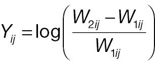

The outcome variable for responder analysis based on a pre-specified absolute change is then given by
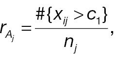


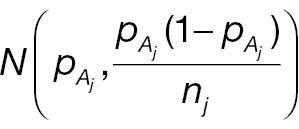

where Φ(·) is the cumulative distribution function (CDF) of a standard normal distribution. The hypotheses for non-inferority testing based on the derived endpoint of absolute change and the corresponding responder analysis can be set up as follows.
Absolute change:
(3)
where δ 1 is the non-inferiority margin in hypothesis testing using absolute change.
Responder analysis based on a pre-specified threshold (improvement) of absolute change:
(4)
where δ 2 is the non-inferiority margin in hypothesis testing using responder analysis.
For a non-inferority test based on the derived endpoint of absolute difference, the Z test statistic under the null hypothesis in Equation (3) is given by

where


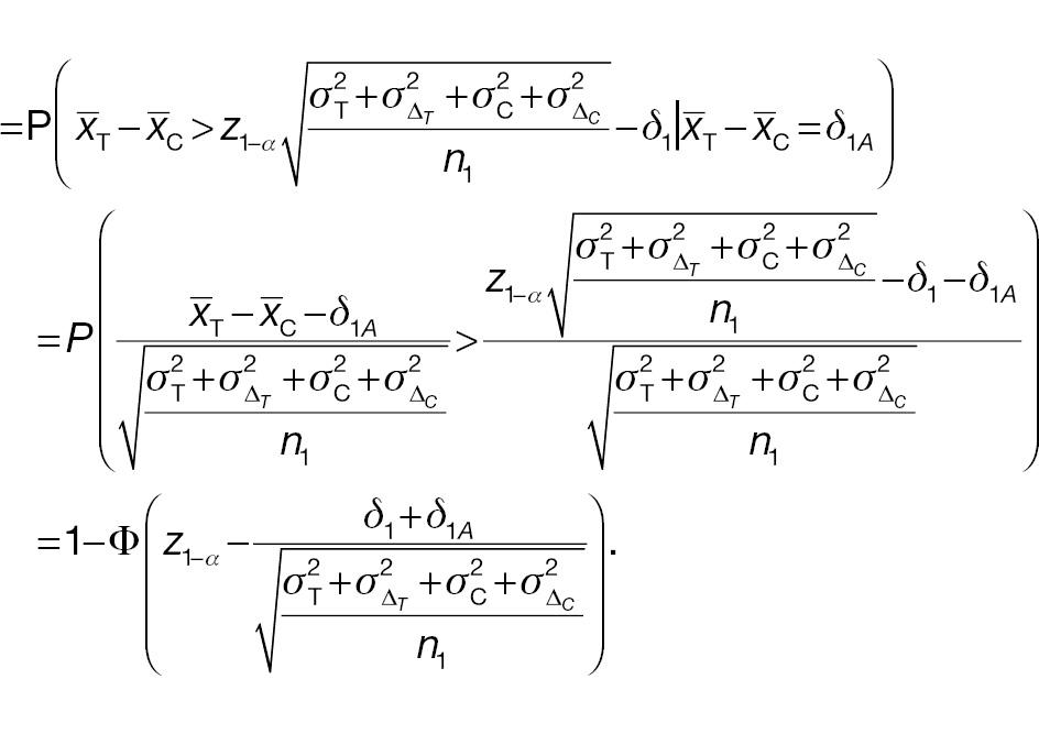
The sample-size requirement for the non-inferiority test using absolute difference can then be obtained as follows:

For a non-inferiority test of responder analysis based on a pre-specified threshold (improvement) of absolute difference, the Z test statistic under the null hypothesis in Equation (4) can be derived as follows:

where


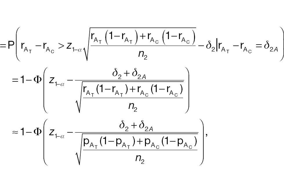
where the last approximate equation holds according to Slutsky’s theorem [1]. The sample-size requirement for a non-inferiority test for responder analysis based on a pre-specified threshold (improvement) of absolute difference is then given by the following:

2.2 Statistical power comparison in non-inferiority tests
Many previous studies have suggested avoiding relative difference because of statistical inefficiency [15]. Extending this idea, we compared statistical power for non-inferiority testing using absolute change and a responder analysis using absolute change. The comparisons of required sample sizes and conclusion for non-inferiority tests are also shown in this section. Let AC denote absolute change and PAC denote responder analysis using absolute change.
From the formula of statistical power of a non-inferiority test shown in Section 2, the power difference can be computed with the CDF of N(0,1). Through Taylor expansion, the CDF of N(0,1) Φ(·) can be written as follows:

Keeping the first term of the Taylor expansion in Equation (11), Φ(x 1) – Φ(x 2) can be simplified as follows:

To compare the statistical power of a non-inferiority test using the absolute-change endpoint with the statistical power for a responder analysis using the absolute-change endpoint, we first simplify


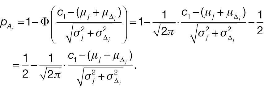
and
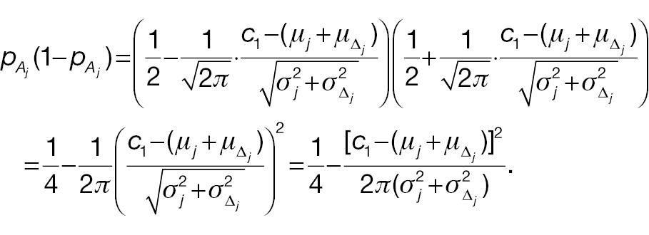
Hence,

and
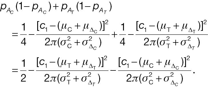
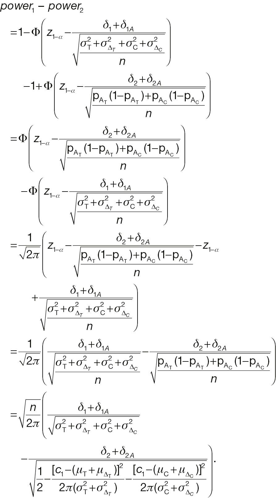
If the sample sizes of a non-inferiority test using absolute change and the corresponding responder analysis are assumed to be the same, denoted n, on the basis of Equation (12), the difference between power 1 and power 2 can be written as follows:
2.3 Sample-size comparison in non-inferiority tests
From Equation (15) and (16), the sample size for the responder analysis using the absolute-change endpoint in Equation (10) can be written as follows:

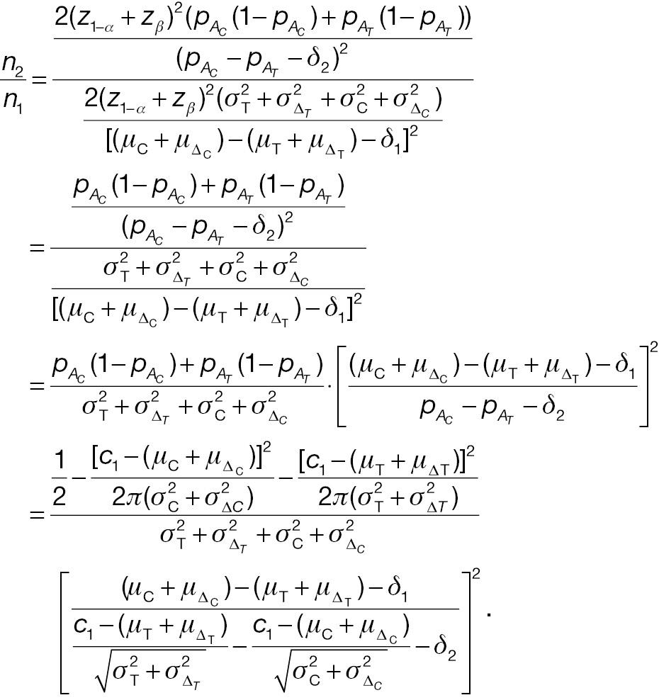
When the significance level and desired statistical power are the same, the necessary sample sizes for a responder analysis and a test from absolute change can be compared with the following ratio:
2.4 Conflict probability in non-inferiority tests
In this section, we investigate the probabilities of a non-inferority test using absolute change as the endpoint and the corresponding responder analysis having similar or different conclusions. We assume that the samples used to conduct these two types of non-inferority test are the same. Thus, four types of events are possible:
Both AC and PAC reject H 0


AC fails to reject H 0, whereas PAC rejects H 0


AC rejects H 0, whereas PAC does not reject H 0


Both AC and PAC do not reject H 0


3. RESULTS
In this section, a numerical analysis using simulated data is conducted to investigate the difference between using absolute change as an endpoint and the corresponding responder analysis in terms of sample-size requirement, statistical power, and non-inferiority-test conclusions. Responses are assumed to follow a normal distribution. The allocation ratio is 1:1. The simulation is conducted 1000 times. Additionally, a case study is used to investigate the difference between a typical non-inferiority test and responder analysis by using real clinical data from [5]. Again, AC denotes a typical non-inferiority test using absolute change as the endpoint, and PAC denotes the corresponding responder analysis. The significance level is 0.05, and the desired power is 0.80.
3.1 Numerical analysis
According to Equation (7), the sample size of AC is associated with the population mean, population variance, and non-inferiority margin. The treatment-group population mean is set to 0.2 or 0.3, the control-group population mean is set to 0, and the population variance of both groups is 1.0, 2.0, or 3.0. Table 1 presents the required sample size of AC to achieve 80% statistical power. The sample size is associated with the effect size and the non-inferiority margin. When the effect size is fixed, a larger non-inferiority margin leads to a smaller sample size in AC; when the non-inferiority margin is fixed, a larger effect size leads to a smaller sample size in AC. Similarly, according to Equation (10), the sample size of PAC is additionally associated with the cut-off value (threshold) used to determine responders. As shown in Table 2 , the influences of effect size and non-inferiority margin on the sample size are the same as in Table 1 when the cut-off value is fixed. However, the influence of the cut-off value on the sample-size calculation is quite complex, because its effects are associated with not only its absolute value but also the population mean and variance.
Sample sizes for non-inferiority tests using the absolute-change endpoint (AC).
 |
 | |||||||||||||||||
|---|---|---|---|---|---|---|---|---|---|---|---|---|---|---|---|---|---|---|
 | 1.0 | 2.0 | 3.0 | 1.0 | 2.0 | 3.0 | ||||||||||||
 | 1.0 | 2.0 | 3.0 | 1.0 | 2.0 | 3.0 | 1.0 | 2.0 | 3.0 | 1.0 | 2.0 | 3.0 | 1.0 | 2.0 | 3.0 | 1.0 | 2.0 | 3.0 |
| δ 1 = 0.25 | 246 | 368 | 490 | 368 | 490 | 612 | 490 | 612 | 734 | 164 | 246 | 328 | 246 | 328 | 410 | 328 | 410 | 492 |
| δ 1 = 0.30 | 198 | 298 | 396 | 298 | 396 | 496 | 396 | 496 | 594 | 138 | 208 | 276 | 208 | 276 | 344 | 276 | 344 | 414 |
| δ 1 = 0.35 | 164 | 246 | 328 | 246 | 328 | 410 | 328 | 410 | 492 | 118 | 176 | 236 | 176 | 236 | 294 | 236 | 294 | 352 |
| δ 1 = 0.40 | 138 | 208 | 276 | 208 | 276 | 344 | 276 | 344 | 414 | 102 | 152 | 202 | 152 | 202 | 254 | 202 | 254 | 304 |
| δ 1 = 0.45 | 118 | 176 | 236 | 176 | 236 | 294 | 236 | 294 | 352 | 88 | 132 | 176 | 132 | 176 | 220 | 176 | 220 | 264 |
| δ 1 = 0.50 | 102 | 152 | 202 | 152 | 202 | 254 | 202 | 254 | 304 | 78 | 116 | 156 | 116 | 156 | 194 | 156 | 194 | 232 |
| δ 1 = 0.55 | 88 | 132 | 176 | 132 | 176 | 220 | 176 | 220 | 264 | 70 | 104 | 138 | 104 | 138 | 172 | 138 | 172 | 206 |
| δ 1 = 0.60 | 78 | 116 | 156 | 116 | 156 | 194 | 156 | 194 | 232 | 62 | 92 | 124 | 92 | 124 | 154 | 124 | 154 | 184 |
| δ 1 = 0.65 | 70 | 104 | 138 | 104 | 138 | 172 | 138 | 172 | 206 | 56 | 84 | 110 | 84 | 110 | 138 | 110 | 138 | 166 |
| δ 1 = 0.70 | 62 | 92 | 124 | 92 | 124 | 154 | 124 | 154 | 184 | 50 | 76 | 100 | 76 | 100 | 124 | 100 | 124 | 150 |
Sample sizes for responder analysis using the absolute-change endpoint (PAC).
 |
 | |||||||||||||||||
|---|---|---|---|---|---|---|---|---|---|---|---|---|---|---|---|---|---|---|
| 1.0 | 2.0 | 3.0 | 1.0 | 2.0 | 3.0 | |||||||||||||
 | 1.0 | 2.0 | 3.0 | 1.0 | 2.0 | 3.0 | 1.0 | 2.0 | 3.0 | 1.0 | 2.0 | 3.0 | 1.0 | 2.0 | 3.0 | 1.0 | 2.0 | 3.0 |
| Cut-off value = 0.1 | ||||||||||||||||||
| δ 2 = 0.25 | 114 | 122 | 126 | 122 | 132 | 136 | 126 | 136 | 142 | 90 | 38 | 100 | 104 | 110 | 114 | 110 | 118 | 122 |
| δ 2 = 0.30 | 86 | 92 | 94 | 92 | 98 | 100 | 94 | 100 | 104 | 70 | 96 | 76 | 80 | 84 | 86 | 84 | 88 | 92 |
| δ 2 = 0.35 | 68 | 72 | 74 | 72 | 76 | 78 | 74 | 78 | 80 | 56 | 74 | 60 | 62 | 66 | 68 | 66 | 70 | 72 |
| δ 2 = 0.40 | 54 | 58 | 58 | 58 | 60 | 62 | 58 | 62 | 64 | 46 | 60 | 50 | 50 | 54 | 54 | 54 | 56 | 56 |
| δ 2 = 0.45 | 44 | 46 | 48 | 46 | 50 | 50 | 48 | 50 | 52 | 90 | 48 | 40 | 42 | 44 | 44 | 44 | 46 | 46 |
| Cut-off value = 0.2 | ||||||||||||||||||
| δ 2 = 0.25 | 114 | 132 | 142 | 114 | 132 | 142 | 114 | 132 | 142 | 90 | 104 | 110 | 96 | 110 | 118 | 100 | 114 | 122 |
| δ 2 = 0.30 | 86 | 98 | 104 | 86 | 98 | 104 | 86 | 98 | 104 | 70 | 80 | 84 | 74 | 84 | 88 | 76 | 86 | 92 |
| δ 2 = 0.35 | 68 | 76 | 80 | 68 | 76 | 80 | 68 | 76 | 80 | 56 | 62 | 66 | 60 | 66 | 70 | 60 | 68 | 72 |
| δ 2 = 0.40 | 54 | 60 | 62 | 54 | 60 | 62 | 54 | 60 | 62 | 46 | 50 | 54 | 48 | 54 | 56 | 50 | 54 | 56 |
| δ 2 = 0.45 | 44 | 48 | 52 | 44 | 48 | 52 | 44 | 48 | 52 | 38 | 42 | 44 | 40 | 44 | 46 | 40 | 44 | 46 |
| Cut-off value = 0.3 | ||||||||||||||||||
| δ 2 = 0.25 | 112 | 142 | 158 | 104 | 132 | 146 | 102 | 126 | 140 | 90 | 110 | 122 | 90 | 110 | 122 | 90 | 110 | 122 |
| δ 2 = 0.30 | 84 | 104 | 114 | 80 | 98 | 106 | 78 | 94 | 104 | 70 | 84 | 92 | 70 | 84 | 92 | 70 | 84 | 92 |
| δ 2 = 0.35 | 66 | 80 | 86 | 64 | 74 | 82 | 62 | 74 | 80 | 56 | 66 | 70 | 56 | 66 | 70 | 56 | 66 | 70 |
| δ 2 = 0.40 | 54 | 62 | 68 | 52 | 60 | 64 | 50 | 58 | 62 | 46 | 54 | 56 | 46 | 54 | 56 | 46 | 54 | 56 |
| δ 2 = 0.45 | 44 | 50 | 54 | 42 | 48 | 52 | 42 | 48 | 50 | 38 | 44 | 46 | 38 | 44 | 46 | 38 | 44 | 46 |
| Cut-off value = 0.4 | ||||||||||||||||||
| δ 2 = 0.25 | 110 | 150 | 176 | 96 | 130 | 150 | 92 | 122 | 140 | 88 | 118 | 134 | 84 | 110 | 124 | 82 | 106 | 120 |
| δ 2 = 0.30 | 84 | 108 | 124 | 74 | 96 | 108 | 70 | 90 | 102 | 68 | 88 | 100 | 66 | 82 | 94 | 64 | 80 | 90 |
| δ 2 = 0.35 | 64 | 82 | 92 | 58 | 74 | 82 | 56 | 70 | 78 | 56 | 68 | 76 | 52 | 66 | 72 | 52 | 64 | 70 |
| δ 2 = 0.40 | 52 | 64 | 72 | 48 | 58 | 64 | 46 | 56 | 62 | 46 | 56 | 60 | 44 | 52 | 58 | 42 | 52 | 56 |
| δ 2 = 0.45 | 42 | 52 | 58 | 40 | 48 | 52 | 38 | 46 | 50 | 38 | 46 | 50 | 36 | 44 | 48 | 36 | 42 | 46 |
A comparison of sample sizes in Tables 1 and 2 indicates that when the non-inferiority margin is fixed, the required sample size of AC is much larger than that of PAC. One important assumption is that the non-inferiority margins of the two tests are the same. The reason for this assumption is that many researchers have suggested using responder analysis as a secondary analysis [3]; i.e., the sample size is computed on the basis of the primary analysis, and statistical analysis of a typical non-inferiority test and the responder analysis are conducted on the same dataset. However, in practice, the non-inferiority margins in these two tests are likely to differ, because these two tests have different meanings. Therefore, when conducting responder analysis is the secondary analysis, the power of the secondary analysis might potentially be insufficient.
Next, we compare the statistical power of AC and PAC by using Equations (6) and (9), when the sample size is fixed. In the simulation process, the sample size used to generate random samples is the minimum of all possible sample sizes, given the population mean and standard deviation. Here, the population means of the treatment and control groups are 0.2 and 0; the population variance of the treatment group is 2; the population variance of the control group ranges from 1 to 3; and the cut-off value ranges from 0.1 to 0.8. To make the power comparable, the non-inferiority margins of AC and PAC are assumed to be the same. As shown in Figure 1 , with a fixed sample size, the statistical power of AC is smallest, thus suggesting that a larger sample size is required to achieve the desired power with AC than PAC. This finding is consistent with the results in Tables 1 and 2 . Additionally, in PAC, the statistical power values when different cut-off values are used become closer to one another as the population variance increases. The statistical power of PAC is either slightly lower than 80% or above 80%, regardless of the cut-off value. The statistical power of AC is always below 60%. Hence, if researchers conduct a sample-size calculation based on responder analysis but ultimately use a typical non-inferiority test, they will not be able to achieve sufficient statistical power.
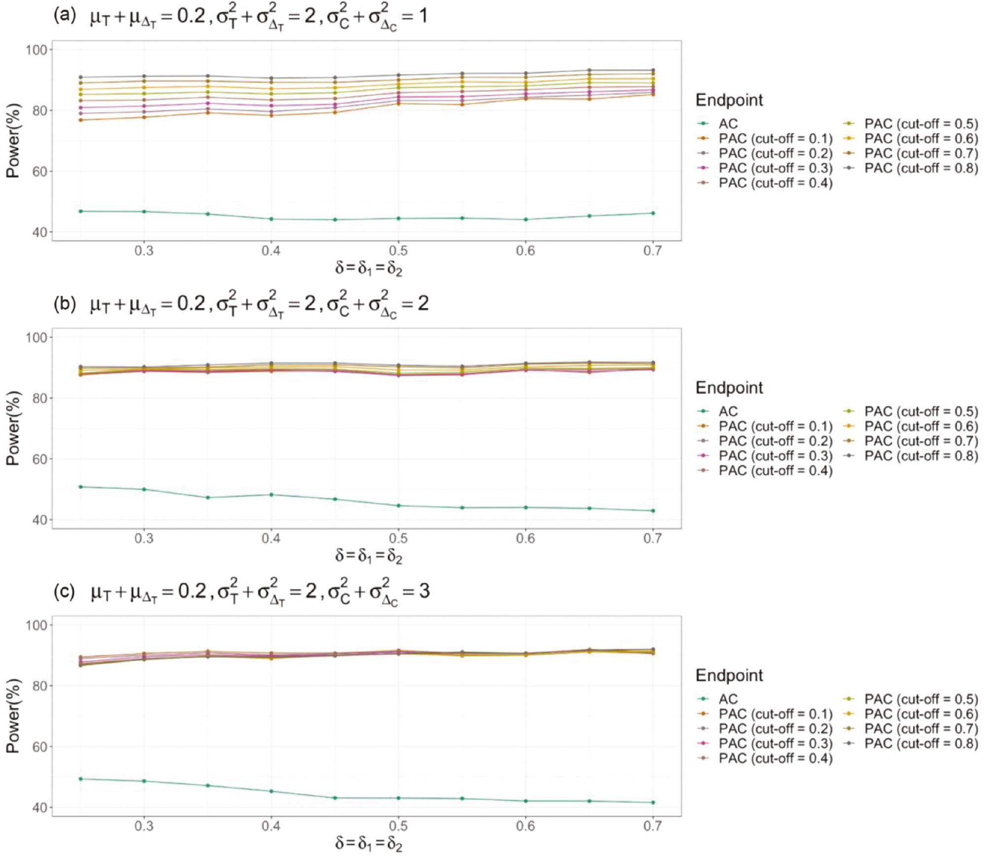
Statistical power comparison of non-inferiority tests using absolute change as an endpoint (AC) and corresponding responder analysis (PAC).
To illustrate the relationships among required sample sizes, we assume that the non-inferiority margins of using the absolute-change endpoint and responder analysis are the same. The setting is the same as that in Figure 1 . In Figure 2 , the ratio of the PAC sample size to AC is used to represent the relationship between the AC and PAC sample size, where N 1 denotes the sample size of AC, and N 2 denotes the sample size of PAC. Under the settings used here, N 2/N 1 is always smaller than 0.35, thus suggesting that the sample size of AC is much larger than that of PAC. When the non-inferiority margin increases, ratios with different cut-off values become not only smaller but also closer to one another. Comparison of Figure 2a–c indicates that the ratio of sample sizes decreases, and the sample-size ratios with different cut-off values become closer to one another when the variance of the control group increases.
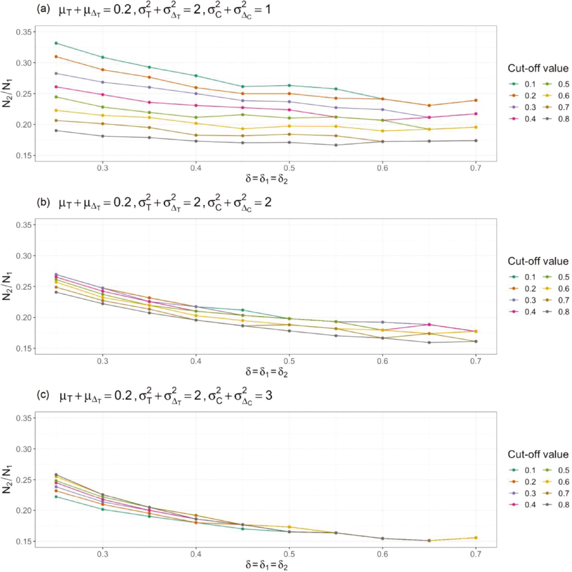
Sample-size comparison of non-inferiority tests using absolute change as an endpoint (AC) and corresponding responder analysis (PAC).
Another essential parameter of interest in responder analysis is the cut-off value (threshold) to determine whether an observation indicates a responder. Let the population mean of the treatment group range from 0.10 to 0.30. To make the results comparable, the non-inferiority margins in AC and PAC are set to 0. The range of the cut-off value is set to be larger than before, from −3 to 3. The simulation process initially randomly generates continuous samples from a normal distribution, where the sample size is computed with the AC sample-size formula in Equation (7). Then, using the cut-off value, we label each participant as either a responder or a non-responder. As shown in Figure 3 , the cut-off value can indeed drive the conclusion in a different direction. In Figure 3a , a negative cut-off value provides conflicting results; in Figure 3b , a more extreme cut-off value provides conflicting results; the same findings are indicated in Figure 3c . Additionally, the influence of the cut-off value on the hypothesis-testing result is associated with the population mean and variance; however, the overall pattern is similar. Hence, a more extreme cut-off value, i.e., a cut-off farther away from the population mean, is more likely to lead to conflicting conclusions.
3.2 Case study
In Section 3.1, we studied the effects of essential parameters on sample-size requirements, statistical power, and test conclusions by using simulated data. To provide a clearer illustration of the influence of the cut-off value on non-inferiority-test results, we conducted a case study using real clinical data from an observational study on rehabilitation in patients who had received lung transplants [5]. That study’s primary aim was to compare the performance of individual rehabilitation and group rehabilitation in participants both pre-operatively and post-operatively, measured by a primary outcome variable of the change in 6MWD (detailed information in Table 3 ).
Changes in 6MWD in pre-operative and post-operative participants in [5].
| Pre-operative | Post-operative | |||
|---|---|---|---|---|
| Rehabilitation | Group | Individual | Group | Individual |
| Sample size | 93 | 81 | 110 | 105 |
| Mean (SD) | 51.6 (81.3) | 56.6 (62.9) | 174 (97.6) | 160 (89.4) |
| Median [Q1, Q3] | 44.5 [6.40,102] | 59.7 [25.0,93.9] | 168 [106, 232] | 159 [104, 208] |
In this section, the non-inferiority test was used to study the circumstances in which AC and PAC may lead to different conclusions. According to previous studies [12, 13], a clinically meaningful change in 6MWD is between 25 m and 33 m. The cut-off value herein ranged from 20 m to 35 m, to provide more comprehensive understanding of the effects of cut-off value selection on study conclusions. The non-inferiority margin of AC ranged from −0.3 to 0.3, and the non-inferiority margin of PAC ranged from 0 to 0.03. As shown in Figure 4 , for pre-operative patients, some cut-off values may lead to different conclusions. For instance, in Figure 4a , a cut-off value larger than 27 yielded conflicting results. However, for post-operative patients, if the cut-off value was between 20 and 35, both AC and PAC always yielded consistent results. Closer examination of the data indicated that, for most post-operative patients, the change in 6MWD was either extremely large (above 35) or extremely small (below 20). That is, in this scenario, an extreme cut-off value (ranging from 20 to 35) did not significantly affect the proportion of responders among post-operative patients. These results suggest that cut-off value selection may cause responder analysis and typical non-inferiority tests to yield conflicting findings under certain circumstances.
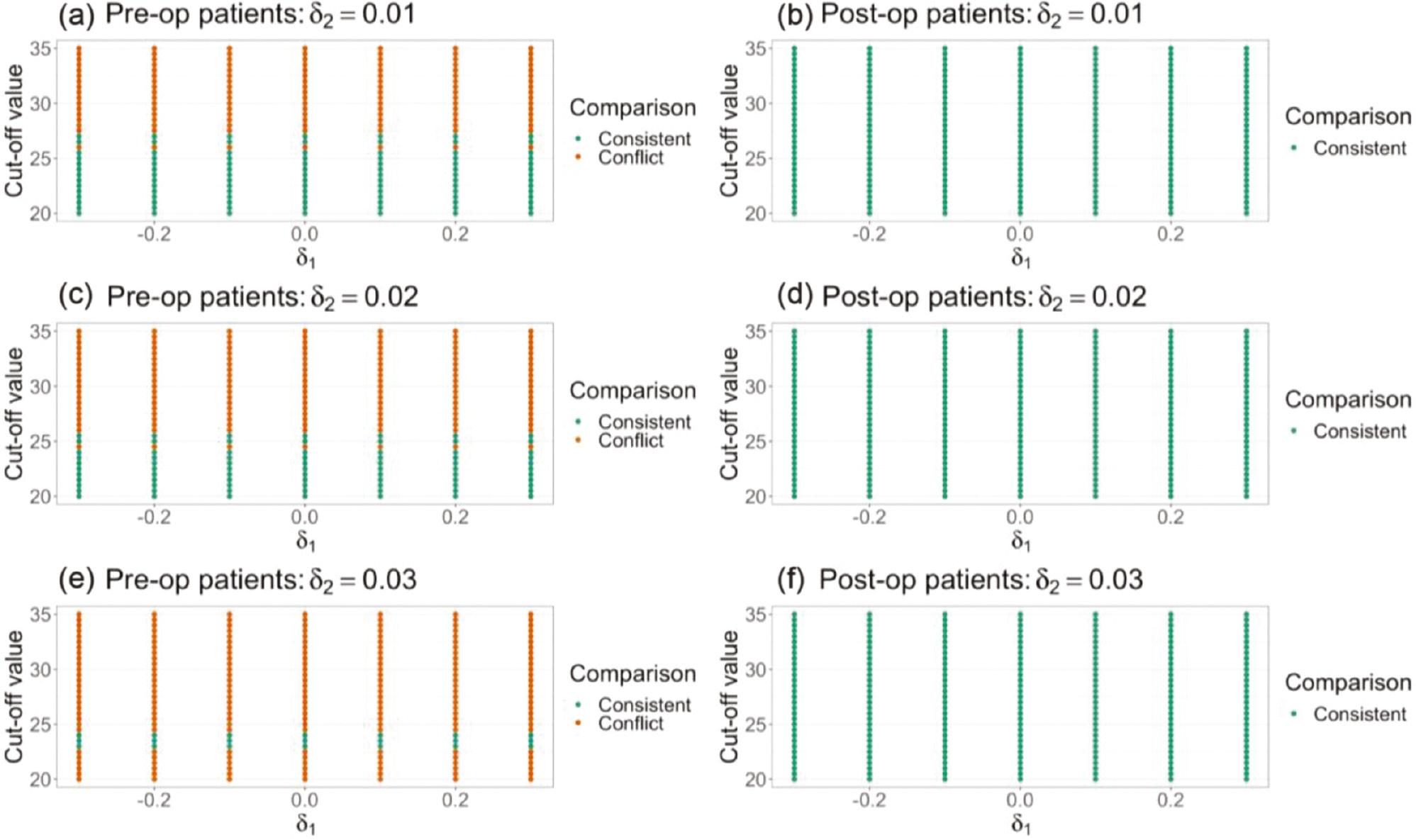
Comparison of non-inferiority-test results of typical tests using absolute change as an endpoint (AC) and corresponding responder analysis (PAC) in a study examining a rehabilitation program after lung transplantation [5].
As described in Section 1, a responder analysis answers a different question from a typical non-inferiority test. Specifically, if an extreme cut-off value is selected, responder analysis investigates whether the test treatment might provide substantial clinical benefits to patients. For example, in Figure 4a , AC yields an insignificant conclusion, i.e., individual rehabilitation is inferior to group rehabilitation, whereas PAC yields a significant conclusion when the cut-off value is large. These findings suggest that individual rehabilitation is non-inferior to group rehabilitation only for a small proportion of patients and provides a benefit of substantial improvement. The large cut-off value allowed us to focus on a smaller proportion of patients with substantial improvement, but this difference may not be detectable in typical non-inferiority tests, thus yielding conflicting findings.
4. DISCUSSION
One of the most important steps in any clinical trial is determining the primary study endpoint, which may influence aspects including establishment of hypotheses, selection of statistical models, and calculation of sample size. In general, four types of study endpoints exist: (i) absolute change, (ii) relative change, (iii) responder analysis using absolute change, and (iv) responder analysis using relative change. To demonstrate a comparison of different study endpoints, this work focused on the comparison of endpoints (i) and (iii) in non-inferiority tests, in terms of the sample-size requirement, statistical power, and whether different endpoints might lead to different conclusions. However, the comparison process in this study could also be generalized to compare any two study endpoints described above.
In the numerical study section, both a simulation study and a case study using data from [5] were conducted. According to the simulation study, the required sample size of a non-inferiority test using AC is associated with the population mean, variance of the treatment and control groups, and non-inferiority margin. The sample size of the corresponding PAC is additionally associated with the cut-off value used to determine responders. After fixing all parameters, we observed that PAC requires a smaller sample size than AC. That is, for the same sample size, PAC will always have greater statistical power than AC, as shown in Figure 1 . When the desired statistical power is the same, the sample-size ratio of PAC to AC is always smaller than 1, an aspect also associated with the non-inferiority margin and cut-off value. However, the effects of these two parameters decrease with increasing population variance. As the cut-off value becomes more extreme, the likelihood of obtaining conflicting conclusions from a non-inferiority hypothesis test increases. This aspect was observed in both the simulation study and the case study. Our findings indicated that the selection of cut-off value selection is highly important, because it may lead to conflicting results when the mean and median in the treatment and control groups are close to the cut-off value.
Without a loss of generalizability, similar conclusions may be found in superiority and equivalence tests. The fundamental reason why typical non-inferiority/superiority/equivalence tests using absolute change as an endpoint and corresponding responder analysis provide conflicting conclusions is the distribution of the target population. If the samples follow a normal distribution, typical tests and responder analysis are highly likely to yield the same conclusion when the cut-off value is close to the population mean. Otherwise, these two types of analysis would provide conflicting results, particularly when the cut-off value is far from the population mean.
Because of the great importance of cut-off value selection and the possibility of obtaining conflict conclusions, we suggest determining cut-off values on the basis of existing knowledge in combination with statistical analysis of the collected sample in conducting responder analysis. Although the clinically important difference (MCID) is always used as the cut-off value [4], some studies have proposed some guidance or approaches for the selection of cut-off values [16, 17]. Additionally, because the sample-size requirements of AC and PAC are different, the sample size must be verified to be sufficiently large to achieve the desired statistical power. Notably, typical tests and responder analysis may require different sample sizes, differ in power, and yield different study conclusions; moreover, tests using absolute instead of relative change as a study endpoint may face the same challenges. Some studies have reported that absolute- and relative-change endpoints may lead to conflicting conclusions [1, 18]. In addition, these endpoints are viewed differently among drug approval administrations. According to the non-inferiority-test guidance from the US Food and Drug Administration (FDA), study constancy is expected to be based on the constancy of relative effects, not absolute effects [19]. However, the European Medicines Agency’s (EMA) guidance uses absolute difference to illustrate instructions for non-inferiority tests [20]. Hence, a drug approved by the FDA might not be approved by the EMA, or vice versa, because the required sample size and statistical power of using absolute change and relative change as a study endpoint differ [1]. Hence, providing the confidence intervals of cut-off values may be useful when a typical non-inferiority test and responder analysis might lead to consistent conclusions. Moreover, the circumstances in which both absolute- and relative-change endpoints provide the same non-inferiority-test results should be investigated.

