Common SNPs explain some of the variation in the personality dimensions of neuroticism and extraversion

There is no author summary for this article yet. Authors can add summaries to their articles on ScienceOpen to make them more accessible to a non-specialist audience.

Abstract

The personality traits of neuroticism and extraversion are predictive of a number of social and behavioural outcomes and psychiatric disorders. Twin and family studies have reported moderate heritability estimates for both traits. Few associations have been reported between genetic variants and neuroticism/extraversion, but hardly any have been replicated. Moreover, the ones that have been replicated explain only a small proportion of the heritability (<∼2%). Using genome-wide single-nucleotide polymorphism (SNP) data from ∼12 000 unrelated individuals we estimated the proportion of phenotypic variance explained by variants in linkage disequilibrium with common SNPs as 0.06 (s.e.=0.03) for neuroticism and 0.12 (s.e.=0.03) for extraversion. In an additional series of analyses in a family-based sample, we show that while for both traits ∼45% of the phenotypic variance can be explained by pedigree data (that is, expected genetic similarity) one third of this can be explained by SNP data (that is, realized genetic similarity). A part of the so-called ‘missing heritability' has now been accounted for, but some of the reported heritability is still unexplained. Possible explanations for the remaining missing heritability are that: (i) rare variants that are not captured by common SNPs on current genotype platforms make a major contribution; and/ or (ii) the estimates of narrow sense heritability from twin and family studies are biased upwards, for example, by not properly accounting for nonadditive genetic factors and/or (common) environmental factors.

Related collections

Most cited references 54

Record: found
Abstract: found
Article: not found

Data and Theory Point to Mainly Additive Genetic Variance for Complex Traits

William Hill, Michael E Goddard, Peter Visscher (2008)

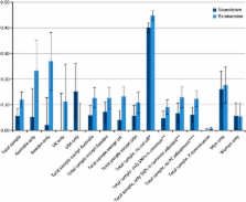
Introduction Complex phenotypes, including quantitative traits and common diseases, are controlled by many genes and by environmental factors. How do these genes combine to determine the phenotype of an individual? The simplest model is to assume that genes act additively with each other both within and between loci, but of course they may interact to show dominance or epistasis, respectively. A long standing controversy has existed concerning the importance of these non-additive effects, involving both Fisher [1] and Wright [2]. Estimates of genetic variance components within populations have indicated that most of the variance is additive [3],[4]. Increasing knowledge about biological pathways and gene networks implies, however, that gene-gene interactions (epistasis) are important, and some have argued recently that much genetic variance in populations is due to such interactions [5],[6],[7],[8]. It is important to distinguish between the observations of dominance or epistasis at the level of gene action at individual loci, exemplified by a table of genotypic values, and the observations of variance due to these components in analysis of data from a population. For example, at a completely dominant locus almost all the variance contributed is additive if the recessive gene is at high frequency [3],[4]. An understanding of the nature of complex trait variation is important in evolutionary biology, medicine and agriculture and has gained new relevance with the ability to map genes for complex traits, as demonstrated by the recent burst of papers that report genome-wide association studies between complex traits and thousands of single nucleotide polymorphisms (SNPs) [9],[10],[11],[12],[13]. Here we attempt to resolve the alternative sources of evidence on the importance of non-additive genetic variation. We evaluate the evidence from empirical studies of genetic variance components and indeed find that additive variance typically accounts for over half and often close to 100% of the total genetic variance. We then present new theory and results that show why this is the case even if there are non-additive effects at the level of gene action. Empirical Evidence for Additive and Non-Additive Genetic Variance Estimation of Genetic Variance The genetic variance V G can be partitioned into additive (V A), dominance (V D), and a combined epistatic component (V I), which itself can be partitioned into two locus (V AA, V AD, and V DD) and multiple locus components (V AAA, etc.) [3],[4],[14],[15],[16],[17]. Estimation of additive and non-additive variance components utilises the observed phenotypic similarity of relatives and the expected contribution of additive and non-additive effects to that similarity [3],[4]. In addition to resemblance due to additive or non-additive genetic factors, relatives may resemble each other due to common environmental effects. In an extremely large data set with very many different kinds of relationships present, it is possible in principle to partition variation into many components using modern statistical methods such as residual maximum likelihood [18] (REML) with the animal model [4],[19],[20]. In practice it is never possible to estimate many variance components with useful precision, however, not least because there is a high degree of confounding: for example, full sibs have a higher covariance for all single and multi-locus genetic components than do half sibs. The coefficients of epistatic components are small (e.g., V AA/16 for half-sibs), so estimates have high sampling error and there is little power to distinguish V A from, say, V AA. Selection, assortative mating, and non-genetic covariances also confound estimates. Consequently, there are few accurate estimates of non-additive variance components but there is indirect evidence. For instance, a narrow sense heritability value (h 2 = V A/V P) of one-half, typical for many traits, implies that dominance, all the vast number of epistatic components, and the environmental component, collectively contribute no more than V A. Similarly if the heritability is only a little less than the repeatability (the phenotypic correlation of repeated measures), all non-additive genetic variances and the permanent environmental variance together comprise this small difference. With these caveats we summarise data of various types. Laboratory Animals and Livestock The extensive data on experimental organisms show a range of heritability, higher for morphological than fitness associated traits, averaging as follows [21]: morphology - 0.46, physiology (e.g., oxygen consumption, resistance to heat stress) - 0.33, behaviour - 0.30, and life history - 0.26. There have been extensive estimates of heritability for traits of livestock. For example, for beef cattle, these averaged: post-weaning weight gain 0.31, market weight for age 0.41, backfat thickness 0.44 [22]. In general for morphological traits, such as carcass fatness, egg weight in poultry or fat and protein content of cow's milk, a heritability of 0.5 or so is the norm, whereas for growth traits or milk yield 0.25–0.35 is more typical [23]. These estimates of heritability from half-sib correlations could be biased upwards by additive epistatic terms, but they can not account for estimates of heritability over 25%. Furthermore, estimates of realised heritability from response to selection [3] are not biased in that way, because epistatic components do not contribute to long term selection response [24], and estimates of realised heritability range up to 0.5 for fat content of mice, for example [25]. There are a number of cases where it can be shown directly that V A contributes almost all of V G and indeed almost all of V P. For bristle number in Drosophila melanogaster, the phenotypic correlation between abdominal segments, which, assuming they are influenced by the same genes, estimates V G/V P, is only a little higher than the heritability, indicating that V A/V G∼0.8 [26]. For finger ridge count (in humans), estimates of heritability are close to one and consistent from different sorts of relatives [27]. Even for lowly heritable traits such as litter size in pigs, the repeatability is little higher than the heritability, implying that most genetic variance is additive [28]. Whilst there is a clear relationship between heritability and type of trait, it should be noted that low heritability does not imply low genetic variance: the evolvability (√V A/mean) is higher for fitness than morphological traits [29], and even for estimates of fitness itself or traits closely related to it, additive genetic variance is present [30],[31]. There are rarely good direct estimates of epistatic or dominance variance because these variance components are usually estimated from full-sibs and therefore confounded with the common environment shared by full sibs. However, if the heritability is high, the space for them is limited. Experiments on inbreeding depression provide some evidence on the importance of non-additive effects. Inbreeding depression implies directional dominance in gene effects but, for a given rate of inbreeding depression, as the number of loci increases and the gene frequencies move toward 0 or 1.0, the dominance variance decreases towards zero. Consequently, the importance of inbreeding depression for traits related to fitness is not evidence that the dominance variance is large. The observed linearity of inbreeding depression with inbreeding co-efficient is easiest to explain with directional dominance but not with DD or higher order epistatic effects because these would cause non-linearity unless they happened to exactly cancel each other out. Twin Studies in Humans In contrast to studies of sibs and more distant relatives, identical twins can provide estimates of V G. The classical twin design of samples of monozygotic (MZ) and dizygotic (DZ) twin pairs has been used extensively to estimate variance components for a wide range of phenotypes in human populations. The primary statistics from these studies are the correlations between MZ pairs (r MZ) and between DZ pairs (r DZ). If twin resemblance due to common environmental factors is the same for MZ and DZ twins then r MZ>r DZ implies that part of the resemblance is due to genetic factors and r MZ>2r DZ implies the importance of non-additive genetic effects. Conversely, r MZ<2r DZ implies that common environmental factors cause some of the observed twin resemblance. Sophisticated variance component partitioning methods to estimate components of additive, non-additive and common environmental effects are used widely [32], but all rely on the strong assumptions that resemblance due to common environmental effects is the same for MZ and DZ twins. Attempts to test this hypothesis have not found any evidence to reject it [33],[34]. Nevertheless, even accepting this assumption about common environmental variance, in the classical twin design there are only two primary statistics and three or more variance components cannot be estimated without making additional assumptions. We summarised the MZ and DZ correlations for a wide variety of phenotypes from published twin studies from a single productive laboratory in Australia (genepi.qimr.edu.au). The criteria were that each study must have more than 100 MZ and more than 100 DZ pairs and that the study subjects were Australian twins. For non-continuous traits, studies were included only if they reported polychoric or tetrachoric correlations. In total, 86 phenotypes qualified of which 42 were clinical measures of quantitative traits (including, for example, blood pressure, biochemical measures in blood, body-mass-index, height, tooth dimensions; a full list of phenotypes is available upon request). The MZ and DZ correlations are summarised in Table 1. The correlations were not separated according to the sex of the individuals in all studies; but for those that did separate the sexes, the overall MZ and DZ correlations were calculated as an average, weighted by the total number of pairs. The distribution of r MZ−2r DZ across all 86 phenotypes is shown in Figure 1. On average the MZ correlation is about twice the DZ correlation across a wide range of phenotypes. If we consider only clinically measured phenotypes and ignore opposite-sex twins then the MZ correlation is clearly less than twice the DZ correlation (Table 1). It is possible but unlikely that the variance due to common environmental factors, assortative mating and non-additive genetic factors exactly cancel each other out by chance. Thus the simplest explanation of the results is that additive variance explains most of the observed similarity of twins and non-additive variance is generally of small magnitude and cannot explain a large proportion of the genetic variance. 10.1371/journal.pgen.1000008.g001 Figure 1 Distribution of r MZ−2r DZ for all traits on human twins. Data are from published papers by N.G. Martin and colleagues of the Queensland Institute of Medical Research, Brisbane (www.genepi.edu.au). Across a wide variety of traits the mean difference between the monozygotic twin correlation and twice the dizygotic twin correlation is close to zero, which is consistent with predominantly additive genetic variance and the absence of a large component of variance due to common environmental effects. 10.1371/journal.pgen.1000008.t001 Table 1 Meta-analysis of MZ and DZ correlations in humansa. Group All phenotypes Clinically measured phenotypes No. traits r No. traits r MZ females 58 0.61 24 0.76 MZ males 48 0.65 24 0.75 DZ females 58 0.34 24 0.45 DZ males 48 0.36 24 0.43 OS pairsb 46 0.29 23 0.36 All MZ 86 0.58 42 0.67 All DZ 86 0.29 42 0.35 MZ−2DZ 86 0.00 42 −0.04 These show the correlations (r) of phenotypes of twins, averaged over ranges of traits estimated in large data sets a Data from published papers by N.G. Martin and colleagues of the Queensland Institute of Medical Research, Brisbane (www.genepi.edu.au) b Opposite sex Model Gene Frequency Distributions In view of the apparent conflict between the observations of high proportions of additive genetic variance (often half or more of the phenotypic variance, and even more of the total genetic variance) and the recent reports of epistasis at quantitative trait loci (QTL) [8], we consider explanations beyond that of simple sampling errors and bias of estimates. We focus particularly on the role that the distribution of gene frequencies may play in the relation between the genetic model and the observed genetic variance components. Genetic variance components depend on the mean value of each genotype and the allele frequencies at the genes affecting the trait [3],[4],[17]. Unfortunately the allele frequencies at most genes affecting complex traits are not known, but the distribution of allele frequencies can be predicted under a range of assumptions. This distribution depends on the magnitude of the evolutionary forces that create and maintain variance, including mutation, selection, drift and migration. As the effects on fitness of genes at many of the loci influencing most quantitative traits are likely to be small, we can invoke theory for neutral alleles to serve as a reference point. An important such reference is the frequency distribution under a balance between mutation and random genetic drift due to finite population size in the absence of selection. If mutations are rare, the distribution of the frequency (p) of the mutant allele is f(p)∝1/p, i.e. approximately L-shaped [2],[35],[36], with the high frequency at the tail being due to mutations arising recently. The allele which increases the value of the trait may be the mutant or ancestral allele, so its frequency has a U-shaped distribution f(p)∝1/p+1/(1−p) = 1/[p(1−p)]. As we shall use it often, we define the ‘U’ distribution explicitly by this formula. For loci at which the mutants are generally deleterious, the frequency distribution will tend to be more concentrated near p = 0 or 1 than for this neutral reference point. As another simple reference point we use the uniform distribution, f(p)∝1, 1/(2N) ≤ p ≤ 1−1/(2N), with N the population size. This approximates the steady state distribution of a neutral mutant gene which has been segregating for a very long time [2], and also has much more density at intermediate gene frequencies than the ‘U’ distribution. Our third reference point is at p = 0.5, as in populations derived from inbred crosses, and is the extreme case of central tendency of gene frequency. These analyses assume a gene frequency distribution which is relevant to no selection. For a more limited range of examples we consider the impact of selection on the partition of variance. We consider a limited range of genetic models, some simple classical ones and others based on published models of metabolic pathways or results of QTL mapping experiments. Uniform: f(p) = 1, assuming N is sufficiently large that the discreteness of the distribution and any non-uniformity as p approaches 1 or 0 can be ignored, i.e. integrated over 0 to 1. This and the ‘U’ gene frequency distributions are, for simplicity, assumed to be continuous. Neutral mutation model (‘U’): f(p)∝1/[p(1−p)]. To standardise the distribution, with population size N assumed to be large, note that Thus , where K∼ln(2N). Genetic variance components are obtained by integration of expressions for the variance as a function of p for a specific model of the gene frequency distribution. For multiple locus models the distribution of all loci is assumed to be identical and there is no linkage disequilibrium. We focus on the contribution of additive genetic variance (V A) to genotypic variance (V G). Genotypic Values Single Locus with Arbitrary Dominance Consider a single biallelic locus with genotypic values for CC, Cc and cc of +a, d and −a, respectively (notation of [3]). Then, from [3] For the uniform distribution of p Hence E(V A) = a 2/3 +d 2/15 and E(V D) = 2d 2/15, giving E(VA)/E(VG) = 1−2d 2/(5a 2+3d 2). For the ‘U’-distribution, assuming N is large, and ignoring terms of O(1/N), the integrals simplify to E(V A)∼(a 2+d 2/3)/K, E(V D)∼d 2/(3K) and E(V A)/E(V G) = 1−d 2/(3a 2+2d 2). Additive × Additive Model without Dominance or Interactions Including Dominance A simple additive × additive epistatic model has these genotypic values: Assuming the frequency of B is p and of C is q, with linkage equilibrium: Mean = M = 2a[pq+(1−p)(1−q)] The average effect of substitution of allele B is given by [37] and hence V A = 2a 2[p(1−p)(1−2q)2+q(1−q)(1−2p)2] = a 2(Hp +Hq −4HpHq ), where H is heterozygosity The AA epistatic effect is given by (αα)BC = ¼ d2 M/dpdq = a. Hence V AA = 4a 2 p(1−p)q(1−q)a 2 = a 2 HpHq and VG = a 2(Hp +Hq −3HpHq ), Uniform: simple integration gives E(V A) = 2a 2/9, E(V AA) = a 2/9, E(V G) = a 2/3 ‘U’: Similarly E(V AA) = a 2/(4K). Hence E(V A)/E(V G) = (2−4/K)/(2−3/K) = 1−1/(2K−3), which → 1 for large K. The residue, if any, is V AA. Duplicate Factor Model A simple epistatic model involving all epistatic components for two loci is the following: For an arbitrary number (L) of loci (i), the genotypic value is a except for the multiple ‘recessive’ homozygote, and for one locus it is complete dominance. For pi = 0.5 at all loci: V G = a 2[(½)2L −(¼)2L ], V A = a 2 L(½)4L−1 and V A/V G = 2L/(22L −1). For two loci, V A/V G = 4/15. Uniform: For two loci, E(V A)/E(V G) = 9/16 and declines to 0 as L increases. ‘U’: For two loci For large N, with two loci E(V A) /E(V G) → 4/5 and for very many loci E(V A) /E(V G) → 0 Complementary Model Another simple epistatic model involving all components is the following: which can also be defined for multiple loci. For two loci, for example, using similar methods it can be shown that: for pi = 0.5, V A/V G = 0.56; with the uniform distribution, E(V A)/E(V G) = 2/3; and with the ‘U’ distribution . Analyses of General Models For two-locus models in which the genotypic values were not functions of simple parameters, the genotypic values were entered as data, and V A and V G calculated as functions of the gene frequencies p and q. Bivariate numerical integration was undertaken using Simpson's rule by computing e.g. V A(p,q)f(p,q) over an (m+1) × (m+1) grid of equally spaced p and q values, taking m = 210 or higher power of 2 as necessary for adequate convergence. Results were computed for some models of metabolic pathways [38],[39] and for some published models obtained from QTL analysis [8]. Results/Discussion Single Locus Model Many general points are illustrated by two simple examples, the single locus model with dominance and the two locus model with AA interaction, so we consider these in more detail. For the single locus model with genotypic values for CC, Cc and cc of +a, d and −a, respectively, V A = 2p(1−p)[a+d(1−2p)]2 and V D = 4p 2(1−p)2 d 2. For d = a, i.e. complete dominance of C, V A = 8p(1−p)3 a 2 and V D = 4p 2(1−p)2 a 2 and thus: at p = 0.5, V A = (2/3)V G; if the dominant allele is rare (i.e. p → 0), V G → 8p and V A/V G → 1, and if it is common, V G → 4p 2 and V A/V G → 0. Note, however, that V G and V A are much higher when the dominant allele is at low frequency, e.g. 0.1, than are V G and V D when the recessive is at low frequency, e.g. p = 0.9. Even for an overdominant locus (a = 0), all genetic variance becomes additive at extreme gene frequencies. Considering now expectations (E) over the frequency distributions, let η 2 = E(V A)/E(V G), an equivalent to narrow sense heritability if V E = 0. For the ‘U’ distribution, η 2 = 1−d 2/(3a 2+2d 2) and for the uniform distribution, η 2 = 1−2d 2/(5a 2+3d 2). Hence, for a completely dominant locus, η 2 = 0.8 and η 2 = 0.75 respectively; whereas V A/V G = 0.67 for p = 0.5. In summary, the fraction of the genetic variance that is additive genetic decreases as the proportion of genes at extreme frequencies decreases (Table 2). 10.1371/journal.pgen.1000008.t002 Table 2 Summary of expected proportion of V G that is V A for different modelsa. Genetic model Distribution of allele frequencies p = ½ Uniform ‘U’ (N = 100)b ‘U’ (N = 1000) Dominance without epistasis d = ½a 0.89 0.91 0.93 0.93 Dominance without epistasis d = a 0.67 0.75 0.80 0.80 Dominance without epistasis a = 0 0.00 0.33 0.50 0.50 A × A without dominance 0.00 0.67 0.87 0.92 Duplicate factor 2 loci 0.27 0.56 0.71 0.75 Duplicate factor 100 loci 0.00 0.00 0.00 0.00 Complementary 2 loci 0.57 0.67 0.74 0.76 a Models defined in Methods section b Population size Two Locus Additive × Additive Model The genotypic values (see Theory section) for the simple AA model for double homozygotes BBCC and bbcc are +2a and for bbCC and BBcc are 0, and all single or double heterozygotes are intermediate (+a). With linkage equilibrium, V A/V G = 1−HpHq /[Hp +Hq −3HpHq ], where the heterozygosities are Hp and Hq at loci B and C. Thus V A/V G → 1 if either locus is at extreme frequency (i.e. p or q → 0 or 1), and equals 0 when p = q = 0.5. If p = q, for gene frequencies 0.1, 0.2, 0.3 and 0.4, V A/V G = 0.88, 0.69, 0.43 and 0.14. For the uniform distribution η 2 = 2/3, and for the ‘U’ distribution, the variances are a function of the population size, because more extreme frequencies are possible at larger population sizes. Thus η 2 = (2−4/K)/(2−3/K), where K = ln(2N), so η 2 → 1 for large K. Any residue is V AA. These two examples, the single locus and A × A model, illustrate what turns out to be the fundamental point in considering the impact of the gene frequency distribution. When an allele (say C) is rare, so most individuals have genotype Cc or cc, the allelic substitution or average effect of C vs. c accounts for essentially all the differences found in genotypic values; or in other words the linear regression of genotypic value on number of C genes accounts for the genotypic differences (see [3], p 117). Hence almost all V G is accounted for by V A. Other Epistatic Models With the ‘U’ distribution, most genes have one rare allele and so most variance is additive. Further examples (Table 2) illustrate this point, including the duplicate factor and complementary models where there is substantial dominance and epistasis. These models show mostly V A for the ‘U’ distribution for a few loci but the proportion of the variance which is additive genetic declines as the number increases. With many loci, however, such extreme models do not explain the covariance of sibs (i.e. any heritability) or the approximate linearity of inbreeding depression with inbreeding coefficient, F, found in experiments [3],[4],[40],[41],[42], or the linearity in response to artificial selection [43]. We also analysed a well-studied systems biology model of flux in metabolic pathways [38],[39],[44] and found again that the expected proportion of V G that is accounted for by V A is large (Table 3). 10.1371/journal.pgen.1000008.t003 Table 3 Examples of expected proportion of V G that is VA in models of flux in linear metabolic pathways with a model flux J∝[Σ i (1/Ei )]−1 for a system with 10 loci in which 8 are invariant wild type and two (B, C) are mutants. Activities Flux relative to wildtype, J BBCC = 1 E(V A)/E(V G) E bb Ecc J BbCc J bbCC J BBcc J bbcc Distribution of allele frequencies 0.5 Unia U100b U1000c 1 0.1 0.92 1 0.53 0.53 0.81 0.86 0.88 0.88 0.5 0.1 0.90 0.91 0.53 0.50 0.81 0.85 0.88 0.88 0.1 0.1 0.86 0.53 0.53 0.36 0.77 0.82 0.86 0.87 0.1 0.01 0.85 0.53 0.09 0.09 0.72 0.79 0.83 0.84 Enzyme activities are Ei = 1 for loci 3 to 8, E BB = E CC = 1, values of E bb and E cc are listed, and heterozygotes are intermediate, e.g. E Cc = ½(1+E cc), assuming gene frequency distributions as in Table 2. Flux modelled as [39]. a Uniform b U-shaped with population size of 100 c U-shaped with population size of 1000 Examples of Models from Highly Epistatic Published QTL Analyses A number of QTL analyses using crosses between populations (some inbred, some selected) have been published in which particular pairs (or more) of loci have been identified to have substantial epistatic effects [8]. We consider examples of the more extreme cases of epistasis found, obtaining variance components by numerical integration. Results are shown in Table 4, for examples from [8] deliberately chosen as extreme. Even so, the proportion of the genetic variance that is additive is high with the ‘U’ distribution, except in the dominance × dominance example. Further, as these examples were selected by Carlborg and Haley and us as cases of extreme epistasis, it is not unreasonable to assume that the real epistatic effects are smaller than their estimates. 10.1371/journal.pgen.1000008.t004 Table 4 Examples of expected proportion of V G that is V A in highly epistatic published QTL analyses assuming gene frequency distributions as in Table 2. Modela Genotypic values E(V A)/E(V G) BBCC BbCC bbCC BBCc BbCc bbCc BBcc Bbcc bbcc Distribution of allele frequencies 0.5 Unib U100c U1000d DomEp 4 10 15 11 8 7 10 8 7 0.05 0.52 0.73 0.78 Co-ad 39.0 38.7 35.7 37.6 38.9 37.7 36.8 39.6 40.4 0.11 0.62 0.81 0.85 D × D 4 13 6 13 7 11 5 13 6 0.00 0.15 0.37 0.42 a Values obtained from tables or by interpolation from Box 1c–e of Carlborg and Haley [8]: key to their nomenclature: DomEp: Dominant epistasis (complex); Co-ad: Co-adaptive epistasis; D × D: dominance × dominance epistasis. b Uniform. c U-shaped with population size of 100. d U-shaped with population size of 1000. Relaxation of Assumptions Expectation of a Ratio of Variance Components The formulae we have given have been for the quantities E(V A), E(V G) and the ratio E(V A)/E(V G). The quantity actually observed is V A/V G = Σ iV Ai /ΣV Gi where the expression denotes the sums over loci (i) of the additive and total genetic variance contributed by each in the absence of epistasis or linkage disequilibrium, or in the presence of these, sums over relevant sets of loci. As, for any locus, or for their sum, in general E(V A/V G) ≠ E(V A)/E(V G), we need to consider the relevance of the quantities calculated. Whilst it would be possible to obtain approximations using statistical differentiation [4], formulae are complicated and invoke an assumption of small coefficients of variation of the quantities which does not always hold. Hence we used Monte Carlo simulation and some examples are given in Table 5. It is seen that, except with very few loci, the bias is not great in using the ratio of expectations. In real situations where many loci of differing effects and frequencies are likely to be involved, the bias is likely to be trivial unless a single locus contributes almost all the variance. 10.1371/journal.pgen.1000008.t005 Table 5 Bias in use of E(V A)/E(V G) rather than E(V A/V G) for some models in Table 2 as a function of Numbers of Loci. Uniform distribution E(V A)/E(V G) E(V A/V G) from simulation Locia 64 16 4 1 a = 1, d = 1 0.750 0.749 0.747 0.734 0.609 a = 0, d = 1 0.333 0.335 0.337 0.348 0.430 A × A 0.667 0.667 0.666 0.660 0.646 Dupl. factor 0.562 0.559 0.549 b b ‘U’ distribution with N = 1000 E(V A)/E(V G) E(V A/V G) from simulation Loci* 64 16 4 1 a = 1, d = 1 0.800 0.798 0.796 0.773 0.561 a = 0, d = 1 0.500 0.502 0.516 0.585 0.800 A × A 0.918 0.918 0.919 0.925 0.945 Dupl. factor 0.746 0.743 0.733 b b a Number of loci for non-epistatic cases (complete dominance a = 1, d = 1, and overdominance a = 0, d = 1), numbers of pairs of loci for two-locus epistatic models (A × A and duplicate factor. b Not computed as V G = 0 in some replicates. Influence of Linkage Disequilibrium (LD) In this analysis we have assumed there is Hardy-Weinberg equilibrium (HWE) and linkage equilibrium among the loci. As departures from HWE are transient with random mating, they can be ignored, but LD can persist, and hence the estimated effects at locus C depend on those fitted at B and vice versa. The effect of LD is to reduce the number of haplotypes that segregate in the population so what would be epistatic variance becomes additive or dominance variance. For example, consider the A × A model and complete LD, i.e. equal frequencies at B and C loci and both loci segregating but with only two haplotypes present. Then only Bc and bC haplotypes are present, and genotypic values are 0 for homozygous classes and a for heterozygotes (‘pure’ overdominance), or only BC and bc haplotypes, with genotypic values 2a for homozygotes and a for heterozygotes (‘pure’ underdominance). In either case variances are the same as for the dominance case with a = 0. Thus LD would lead to attribution of real epistatic variance to additive or dominance variance, and would exacerbate the results obtained from discussions of gene frequency distribution. Consequences of Multiple Alleles In these models we have considered solely biallelic loci, appropriate for low mutation rates. Multiallelic loci, in terms of their effects on the trait, can arise from mutations at different structural or control sites. Predictions are complicated by the need to consider k(k−1)/2 genotypic values at a k allelic locus, and many further epistatic terms, so we consider two extreme cases. If the alleles all have similar effects, for example due to a knock-out, the effective mutation rate is increased, but it would require very many such sites for the distribution of frequencies of the trait alleles to differ greatly from proportionality to 1/[p(1−p)]. Such segregation of multiple alleles will be more common in large populations, where in any case the frequency distribution is most extreme, and so the impact is unlikely to be large. A second case is where all alleles have different effects and dominance interactions. Any allelic substitution then produces a change in the mean and so additive variance is present and for example, contributes more V A than does the overdominance model at p = 0.5. Alternative Models The analysis we have given for estimating effects of dominance and epistasis is for the classical method using simple averages over genotypes weighted by their frequencies, which are the least squares estimates in the balanced case and the basis for the analysis of variance [14],[15],[16]. There are alternative parameterisations aimed at exemplifying more clearly the nature of the interactions, including that of ‘physiological epistasis’ [45]. Whilst such alternatives may be of use in the analysis and interpretation of gene or QTL mapping experiments where individual genotypes can be identified or predicted from linked markers, such alternative parameterizations are not feasible in analysis of populations using data solely on the quantitative traits, from which the estimates of genetic variance components and heritability are obtained. Further, as has been pointed out [46], although the estimated effects may differ, the variances explained by different models are generally the same in segregating populations. Effects of Selection on Gene Frequency Distributions and Partition of Variance The ‘U’ and indeed uniform gene frequency distributions are limiting cases applying in the absence of selection on loci affecting the quantitative trait. The results for a wide range of models can be summarised as follows: gene frequencies that cause V A/V G to be small also cause V G to be small. Consequently, when V A and V G are summed over a full range of frequencies, V A/V G is large. This conclusion is dependent on the distribution of gene frequencies being symmetrical, so that cases with large V G and large V A/V G are as common as cases with small V G and small V A/V G. The impact of selection will depend on how it acts on the trait or traits analysed and also on other aspects of fitness, so we need to consider whether the findings are robust to selection. Stabilising selection on the trait, such that individuals with phenotype closest to an optimum are most fit, leads to maintenance of the population mean at or close to the optimum, so that mutants are at a disadvantage if they increase or decrease trait values. Consequently the gene frequency distribution is still broadly U-shaped, but with much more concentration near 0 or 1 [47]. Hence such selection is likely to increase proportions of additive variance. This conclusion would be wrong if there was widespread overdominance at the level of individual genes because this would push gene frequencies to intermediate values. However, the observed inbreeding depression is incompatible with widespread overdominance [48]. Under the neutral mutation or stabilising selection models where gene frequency distributions have extreme U shape, subsequent directional selection will lead to either rapid fixation or increase to intermediate frequency of genes affecting the trait. Even if the distribution of allele frequencies is initially symmetric, a net increase in variance over generations might thus be expected [49] (Chapter 6). Accelerated responses to artificial selection have not been seen, however, in lines founded from natural populations [50]. Calculations show that if genes are analysed independently such an increase in variance with artificial selection can in theory occur following the neutral model only if most gene effects are large (unpublished) or with more extreme frequency distributions following stabilising selection [51]. These ignore the build up of negative gametic disequilibrium through the Bulmer effect [52], however, whereas in simulated multi-locus models of Drosophila no increase in variance was found [51]. Linkage effects would be weaker in species with more chromosomes, but selection lines in these have typically not been founded directly from natural populations. Other types of selection do lead to an asymmetrical distribution of allele frequencies because the unfavourable allele will typically be at a low frequency. We have considered the case of genes whose effect on both the trait measured and on fitness shows complete dominance. Thus recessive and dominant favourable and unfavourable mutants were considered, and their expected contribution to variance computed during their lifetime to fixation or loss, using transition matrix methods. Results are given in Table 6 for population size (N) 100 and selective values (s) of the homozygote of 0.05 (Ns = 5), but the qualitative result is not affected by using weaker or stronger selection. Deleterious, recessive mutations show the lowest V A/V G but even here it is 0.44 and these cases also show the lowest total variance. Consequently, in a trait affected by a mix of genes with varying types of gene action, V A/V G is likely to be well above 0.5. 10.1371/journal.pgen.1000008.t006 Table 6 Expected variance contributed by mutant genes before fixation for population size 100, specified dominance on the quantitative trait (a vs d) and selective (dis)advantage (s in heterozygote and homozygote)a. Model s(het) s(hom) a d E(V G) E(V A)/E(V G) Neutral dominant 0 0 1 1 0.388 0.86 Neutral recessive 0 0 1 −1 0.166 0.66 Neutral randomb 0 0 1 1 or −1 0.277 0.80 Deleterious dominant −0.05 −0.05 1 1 0.145 0.97 Deleterious recessive 0 −0.05 1 −1 0.052 0.44 Advantageous dominant 0.05 0.05 1 1 0.375 0.74 Advantageous recessive 0 0.05 1 −1 0.151 0.71 a e.g., if the mutant gene is completely recessive for the trait and for fitness, d = −a and s(hom) = 0. b Equally likely to be completely dominant or recessive mutants, hence values as in Table 2. Thus if the highest and lowest genotypic values correspond to multiple homozygous classes, it is clear that a high proportion of the variance is expected to be additive genetic even with selection. The potential exceptions occur when there is a maximum at intermediate frequencies, such as with an overdominant locus or some of the cases shown in Table 4. Nevertheless, few confirmed cases of clear overdominance/heterozygote superiority have been found (other than sickle cell anaemia) and the patterns in Table 4 are somewhat erratic. Effect of Population Size and Bottlenecks The theoretical analysis has been undertaken for large populations but much of the experimental data comes from livestock, laboratory animals and humans, all of which have experienced bottlenecks of reduced effective population size. As has been much explored, bottlenecks of population size are likely to change the proportion of variation that is additive, and for example to increase levels of V A for recessives at low frequency [53] and to ‘convert’ epistatic into additive variation [54],[55],[56],[57],[58], thereby increasing the ratio V A/V G. For example, for the additive × additive two locus model, the ratio of variances at inbreeding level F in terms of values at F = 0 is V A(F)/V G(F) = (V A+4FV AA)/(V A+V AA+3FV AA) for any gene frequency (using results of [54], but for loci with dominance or dominance interactions, V A(F)/V G(F) depends on gene frequency. This occurs because the bottleneck leads to the dispersal of gene frequencies and the reduction in mean heterozygosity, so for the AA model, if frequencies are initially intermediate (e.g. 0.5) there is a substantial increase in V A/V G, whereas if frequencies initially follow the ‘U’ distribution, there is little V AA initially, total variance falls and the level of dispersion and V A/V G do not increase appreciably. Indeed, for a population that starts with the gene frequency distribution U-shaped, the loss of heterozygosity is due to fixation. Among the genes that remain segregating the distribution of gene frequencies flattens considerably, and in the absence of new mutation approaches the uniform distribution which has a lower ratio of V A/V G than the ‘U’ distribution. However, despite this, V AA declines faster than V A because, as loci become fixed, the number of pairs of segregating loci declines faster than the number of segregating loci. Thus it is not obvious what effect the bottlenecks in livestock, laboratory or human populations have had on the ratio V A/V G. We suspect it has not been large because, if a large reduction in heterozygosity had occurred, these populations would show low genetic variance and there is no indication that this is the case. In any case, the results show that the conclusion that most genetic variance is additive is fairly robust to assumptions about the distribution of gene frequencies, for instance the ‘U’ and uniform distributions both lead to qualitatively the same conclusion. Evidence for the Effect of Gene Frequency on Variance Components A test of the hypothesis that the lack of non-additive variance observed in populations of humans or animals is because gene frequencies near 0.5 are much less common than those more extreme, not because non-additive effects are absent, is to compare variance components among populations with different gene frequency profiles. For crops such as maize and for laboratory animals, estimates can be got both from outbreds and from populations with gene frequencies of one-half derived from crosses of inbred lines. There are a limited number of possible contrasts and linkage confounds comparisons of variation in F2 and later inter se generations, however, so it is difficult to partition variation between single locus and epistatic components (e.g. [17] ch. 7). The most extensive data are on yield traits in maize. The magnitudes of heritability and of dominance relative to additive variance estimated for different kinds of populations in a substantial number of studies (including 24 on F2 and 27 on open-pollinated, i.e. outbreds) have been summarised [59]. Average estimates of h 2 were 0.19 for open-pollinated populations, 0.23 for synthetics from recombination of many lines, 0.24 for F2 populations, 0.13 for variety crosses and 0.14 for composites. Estimates of V A/V G (from tabulated values of V D/V A [59]) were 0.57, 0.55, 0.50, 0.42 and 0.43, respectively, which are inconclusive but indicate relatively more dominance variance at frequencies of 0.5. Analyses of the magnitude of epistasis at the level of effects, rather than variance, do not provide consistent patterns. For example, in two recent analyses of substantial data sets of F2 populations of maize, one found substantial epistasis [60] and the other almost none [61]. In an analysis of a range of traits in recombinant inbred lines, F2 and triple test crosses [62] in Arabidopsis thaliana, there was substantial additive genetic and dominance variance for all traits, with most estimates of V D/V A in the range 0.3 to 0.5, essentially no significant additive × additive epistatic effects, but several cases of epistasis involving dominance [63]. Although there does appear to be more dominance variance in populations with gene frequencies of one-half than with dispersed frequencies, from these results we cannot reject or accept the hypothesis that there is relatively much more epistatic variance in such populations. One explanation is indeed that there is not a vast amount of epistatic variance in populations at whatever frequency, although another is that maize has unusually small amounts of epistasis. Many additive QTL were identified in an analysis of a line derived from the F2 of highly divergent high and low oil content lines from the long term Illinois maize selection experiment, but with almost no evidence of epistasis or indeed dominance effects [64]. In contrast, an F2 of divergent lines of long-term selected poultry and an F2 from inbred lines of mice showed evidence of highly epistatic QTL effects for body weight [65],[66]. We do not claim to understand these different results, but as has been pointed out [67],[68], QTL with significant epistatic interaction effects might not represent the majority of QTL with small effects contributing to gene networks. Conclusions and Consequences We have summarised empirical evidence for the existence of non-additive genetic variation across a range of species, including that presented here from twin data in humans, and shown that most genetic variance appears to be additive genetic. There are two primary explanations, first that there is indeed little real dominant or epistatic gene action, or second that it is mainly because allele frequencies are distributed towards extreme values, as for example in the neutral mutation model. Complete or partial dominance of genes is common, at least for those of large effect; and epistatic gene action has been reported in some QTL experiments [8],[69]. Detailed analyses in Drosophila melanogaster, using molecular and genetic tools available for it, identify substantial amounts of epistasis, including behavioural traits [70] and abdominal bristle number [71], yet most genetic variation in segregating populations for bristle number appears to be additive (as noted above). But many QTL studies of epistatic gene action suffer from a high degree of multiple testing, increasingly so the more loci and orders of interaction are included, such that they may be exaggerating the amount of epistasis reported. On the assumption that many of the effects are indeed real, we have turned our attention to the second explanation. The theoretical models we have investigated predict high proportions of additive genetic variance even in the presence of non-additive gene action, basically because most alleles are likely to be at extreme frequencies. If the spectrum of allele frequencies is independent of which are the dominant or epistatic alleles, V A/V G is large for almost any pattern of dominance and epistasis because V A/V G is low only at allele frequencies where V G is low, and so contributes little to the total VG . The distribution of allele frequencies is expected to be independent of which are the dominant or epistatic alleles for neutral polymorphisms; but under natural selection the favourable allele is expected to be common and lead to high or low V A/V G depending on whether it is dominant (low V A) or recessive (high V A). The equivalent case for epistasis is that all genotype combinations except one is favourable (low V A) vs. only one genotype combination is favourable (high V A). If genetic variation in traits associated with fitness is due almost entirely to low frequency, deleterious recessive genes which are unresponsive to natural selection, these traits would show low V A/V G. However, neither the empirical evidence nor the theory supports this expectation. There seems to be substantial additive genetic variance for fitness associated traits [21] and fitness itself [30],[31],[72]. Although heritabilities for such traits may be low, they show high additive genetic coefficient of variation (evolvability) [29], and the correlation of repeat records is typically little higher than the heritability (e.g., litter size in pigs), indicating that V A/V G is one-half or more. In agreement with this, when the life history of deleterious, recessive mutants was modelled, V A/V G was found to be 0.44 (Table 6), basically because rare recessives contribute so little variance, albeit most is V D, in non-inbred populations. We believe we have a plausible gene frequency model to explain the minimal amounts of non-additive genetic and particularly epistatic variance. What consequences do our findings have? For animal and plant breeding, maintaining emphasis on utilising additive variation by straightforward selection remains the best strategy. For gene mapping, our results imply that V A is important so we should be able to detect and identify alleles with a significant gene substitution effect within a population. Such variants have been reported from genome-wide association studies in human population [9],[10],[11],[12],[13]. Although there may well be large non-additive gene effects, the power to detect gene-gene interactions in outbred populations is a function of the proportion of variance they explain, so it will be difficult to detect such interactions unless the effects are large and the genes have intermediate frequency. Thus we expect that the success in replicating reported epistatic effects will be even lower than it is for additive or dominance effects, both because multi-locus interactions will be estimated less accurately than main effects and because they explain a lower proportion of the variance. Finally, if epistatic effects are real, gene substitution effects may vary widely between populations which differ in allele frequency, so that significant effects in one population may not replicate in others.

0 comments Cited 351 times – based on 0 reviews      Review now

Bookmark

Record: found
Abstract: found
Article: not found

Assumption-Free Estimation of Heritability from Genome-Wide Identity-by-Descent Sharing between Full Siblings

Peter Visscher, Sarah E. Medland, Manuel A. R Ferreira … (2006)

Introduction The theoretical basis for the resemblance between relatives due to genetic factors was developed by R.A. Fisher in a now famous and classic paper that reconciled Mendelian and biometrical genetics [1]. Following that theoretical basis, quantitative genetic parameters are estimated from the resemblance between different types of relatives by equating the observed phenotypic covariance to the degree of genetic relationship, which is estimated from pedigree data. The degree of relationship is usually expressed as the coefficient of kinship [2] or the additive coefficient of relationship [2,3]. In a non-inbred population, the coefficient of relationship is the expected proportion of alleles identical-by-descent (IBD) between relatives and determines the additive genetic covariance between a pair of relatives. Maximum likelihood (ML) methods and software have been developed to estimate genetic (co)variances in simple [4] and large complex pedigrees [5–7], for univariate and multivariate models. What all these methods have in common is that they estimate genetic parameters from observed variation between and within families, assuming an underlying model for causative components of variance [3]. For example, in twin studies it is commonly assumed that the variance between families is due to common environmental and additive genetic effects, and that the variance within families reflects individual environmental effects (for monozygotic [MZ] pairs) or both individual environmental and additive genetic effects (for dizygotic [DZ] pairs). In human populations, the interplay of genetic, environmental, and cultural factors that cause family resemblance is complex; and crucially, the ultimate separation of nature and nurture effects can generally not be tested empirically through controlled experiments. If the true (unknown) effects causing between-family variance deviate from the assumed model of family resemblance, then the resulting estimates of genetic parameters, and their estimated standard errors (SE), will be biased. This bias could be severe if strong assumptions are necessary to estimate genetic parameters. In the classical twin design, only three underlying parameters are estimated, and strong assumptions regarding the causes of familial resemblance are necessary. For example, the assumption that twin resemblance due to common environmental effects is the same for MZ and DZ pairs is often made. Although some of these assumptions can and have been tested empirically [8,9], the use of twin data to estimate heritability, in particular for traits such as cognitive function, has been controversial [10]. Until now, it has been impossible to exclude a possible confounding between genetic and non-genetic causes of family resemblance. We propose an alternative approach to estimate genetic variance that is based upon the observed proportion of the genome that is shared by relatives and does not make any assumptions about the variation between families. The actual genome-wide relationship, defined as the proportion of the genome that two relatives share IBD, varies around its expectation because of Mendelian segregation [11–14], except for MZ twins and parent-offspring pairs. We use the term “actual” throughout, but other possibilities are “realized relationships” or “the proportion of the genome-shared IBD.” It is possible to estimate this relationship with the use of genetic markers. If these estimates are accurate, then it is, in principle, feasible to estimate genetic parameters within families, obviating the need for contentious assumptions about the sources of between-family variation. In this study, we estimated heritability for height in humans without making any assumptions regarding the causes of resemblance between relatives. We present the relevant theory and estimate the heritability of height from collections of 3,375 full-sib pairs, using genome-wide estimates of actual additive genetic relationships. Bias and accuracy of our estimation approach was explored analytically and by computer simulation. Ours is the first example of an estimate of heritability in humans for which a possible confounding between nature and nurture can be excluded. Results Simulated Data We first assessed bias and accuracy of the estimates of variance components from our method using simulation studies and analytical predictions (see Materials and Methods). Table 1 shows the empirical mean and SE of the ML estimate of the heritability from actual relationships between sibling pairs and statistical power, and their theoretical predictions, for a range of population parameters. As predicted by theory (see Materials and Methods), the SE of the estimates are large, unless the number of pairs is large (10,000), the heritability is large (>0.6), or there is no residual family effect. For 2,500 sib pairs, the SE of the heritability is approximately 0.2 when the true value is 0.8. For 10,000 sib pairs, the range of SE is from 0.08–0.19. The theoretical predictions are accurate, in particular for the special case when the proportion of variance due to non-genetic family effects (f2) is zero. When the proportion of variance due to non-genetic family effects is zero, the estimate of the heritability is biased downwards, in particular when the sample size is small (Table 1). This is because we constrain variance components to be non-negative in our ML estimation procedure. An analytical prediction of the bias is given in Materials and Methods. When the heritability is large (0.8), its estimate is biased downwards, even when the proportion of variance due to non-genetic family effects was larger than zero. Again this is the result of ML estimation, because the sum of the proportion of variance due to genetic and non-genetic factors cannot be larger than unity. Data Application There were a total of 4,401 quasi-independent sibling pairs with estimates of genome-wide IBD sharing statistics. The average proportion of the genome-shared IBD between the sib pairs (the coefficient of additive genetic variance) was 0.498 (SE 0.0005, standard deviation [SD] 0.036), with a range of 0.374–0.617. The distribution of the genome-wide additive coefficients is shown in Figure 1. The mean and range of the proportion of the genome for which a sibling pair shared two alleles IBD (the coefficient of dominance variance, also termed IBD2) was 0.248 (SE 0.0006, SD 0.040) and 0.116–0.401, respectively. Hence, both mean sharing statistics were slightly lower than the expected values of 0.50 and 0.25, respectively. When comparing the mean sharing statistics to their SE, there was evidence for a small but significant departure from expectation (p = 0.002 and 0.0002, for genome-wide additive and dominance coefficients, respectively, assuming a normal distribution of the test statistic). However, the SE is under-estimated because not all pair-wise sib comparisons are independent, so that the departure from expectation is less significant than it appears from the reported p-values. The SD of the mean (additive) IBD and mean IBD2 (dominance) sharing proportions were 0.036 and 0.040, respectively. One quality control measure of our IBD calculations is to test for independence of chromosome-specific additive and dominance relationships. For the combined dataset, 8/231 and 2/231 Spearman rank correlations of the mean IBD sharing between chromosomes were significant at the 0.05 and 0.01 level, respectively, when 12 and 2 were expected under the assumption of independent segregation. For IBD2 sharing the corresponding numbers were 9/231 and 1/231. The observed numbers are not significantly different from expectation under the null hypothesis of independent segregation of chromosomes (the SD of the number of significant correlations at the 0.05 and 0.01 level under the null hypothesis is 3.3 and 1.5, respectively). Figure 2 shows the empirical variance of genome-wide mean IBD and IBD2 sharing, relative to the expected value from theoretical considerations (see Materials and Methods). There is a remarkably good agreement between theory and data, with a correlation between the theoretical and empirical SDs across chromosomes of 0.98 for both mean IBD sharing and mean IBD2 sharing. The correlation between mean IBD and mean IBD2 sharing for 4,401 pairs was 0.91, close to the theoretical value of 0.89 (Figure 3). This large correlation implies a strong sampling correlation between the estimates of additive and dominance variance. ML estimators of heritability are shown in Table 2 for the two datasets separately and for the combined dataset. For each dataset, two models were fitted: a full model (FAE), containing a non-genetic family effect (F), a genome-wide additive effect (A), a residual error effect (E); and a reduced model containing F and E effects only (FE). In all analyses, the estimate of the residual family component was zero, and the estimate of heritability 0.8. For the combined dataset (n = 3,375 pairs), the 95% confidence interval (CI) was from 0.46 to 0.85 (a SE of approximately 0.1) with strong statistical support (p = 0.0003) for a variance associated with genome-wide IBD. The SE of the estimated proportion of variance due to additive genetic variance (h2) is large relative to the estimate. However, because the sampling correlation of the estimates of the non-genetic and genetic variance is large and negative, the estimate of the total proportion of variance explained by genetic and non-genetic effects (i.e., the predicted MZ correlation) is more accurate. For the combined dataset, the ML estimate of this proportion is 0.80, with a 95% CI of 0.62–0.85. Hence, we have estimated the equivalent of an MZ correlation without having such pairs in our data. The estimates from the FE model reflect the sibling correlation of 0.40 and 0.39 for the adolescent and adult datasets. Estimates of the proportion of variance due to additive genetic effects from the AE model (not shown in Table 2) were very close to twice the estimates of the proportion of variance due to the family effect in the FE model. When genome-wide dominance was fitted in addition to F and A, the log-likelihood did not increase significantly for the combined dataset (unpublished data). However, there is unlikely to be sufficient power to distinguish these components with our sample size, consistent with our observed correlation coefficient of 0.89 between the additive genetic and dominance coefficients (Figure 3). Discussion We have shown that it is feasible to estimate genetic parameters solely from segregation within families, without making any assumptions regarding an underlying model for between-family effects. In fact, our only assumption in the analysis is that the additive genetic covariance between relatives is proportional to the actual proportion of the genome that is shared IBD. The resulting estimates of the heritability for height (0.80, 95% CI, 0.46–0.85) and residual family effects (0.00, 95% CI, 0.00–0.17) are very close to estimates from twin studies [15], where the information comes from the difference in correlation between MZ and DZ twin pairs. Essentially, we have estimated the same parameters from DZ and full-sib pairs only. Previously, methods have been proposed to estimate kinship and genetic parameters from marker data when pedigree data are not available, for example, in natural populations [16–18]. Relationship estimation and reconstruction in these methods are based upon identity-by-state sharing of marker alleles. These methods have the same principle as our approach, i.e., first estimating kinship from marker data and subsequently estimating genetic variance from the association between phenotype similarity and estimated kinship. However, there are some important differences between the methods. Firstly, our method is based upon IBD sharing, i.e., we know the pedigree and estimated actual relationships from marker data conditional on the pedigree. The resulting estimates of actual kinship are unbiased and have lower error variance, provided that the pedigree is correct. Secondly, we estimate genetic variance free from possible confounding with environmental factors. In natural populations, even if the kinship were to be estimated without error, there can still be a confounding between genetic and environmental similarities and this could lead to bias. We do not suggest that all estimation of genetic (co)variance from classical designs that utilize between-family comparisons should be abandoned. On the contrary, such designs, for example, those employing twin families, are in principle powerful enough to separate genetic and non-genetic causes of family resemblance if the statistical models are correct or at least a good approximation of the true underlying causes of variation. With sufficient data, our approach allows the testing of hitherto untestable underlying assumptions in other models and, for large samples, allows the estimation of non-additive genetic variation for disease susceptibility and quantitative traits. Therefore, the two methods should be seen as complementary. There is a continuum in the estimation of genetic parameters from genome-wide IBD sharing to quantitative trait loci (QTL) mapping. In QTL mapping, variation in IBD sharing is maximal but many estimations/tests are performed. For sib pairs, the variance of IBD sharing at a single location is 1/8 [14,19–21], whereas it is only 0.0392 genome-wide. Hence, relative to the mean there is about 82 times more variation in IBD sharing between sib pairs at a particular locus than in the genome-wide average [22]. The disadvantage of QTL mapping is that a genome-wide search is performed at many correlated locations, whereas the estimation of genetic variance from genome-wide IBD sharing is a single estimate. An intermediate between the two is to estimate the proportion of additive genetic variance associated with a chromosome [23–25]. The variance in proportion of a chromosome-shared IBD is intermediate between the sharing proportion at a single location and genome-wide, as shown in Table 3. We note that the emphasis in this study is on the estimation of genetic parameters rather than its detection. Hence, in contrast to QTL mapping where hypothesis testing and p-values are important, we have concentrated on the sampling variance of the estimated parameters, because for most traits it is usually known that there is genetic variance, and the scientific question is what proportion of observed variation is genetic. Although our estimates of the variation in mean IBD and IBD2 sharing per chromosome are very similar to the theoretical values (Figure 2) and consistent with recently reported genome-wide sharing statistics from a sample of 498 sib pairs [22], a few caveats are required. Firstly, the theoretical value may be too low for the true variance in IBD sharing on a chromosome because in reality there may be more crossovers than modeled [13,14]. Secondly, the empirical variance of IBD sharing is likely to be an underestimate because the marker information was not perfect. If we assume that our genome-wide average multipoint marker information content was approximately 80%, then we would expect to find a regression slope of the empirical on theoretical SD in IBD sharing of √ 0.80 = 0.89, close to the observed value of 0.92 (Figure 2A). Nevertheless, the correlations of 0.98 between empirical and theoretical values are extremely high. We detected a small genome-wide deviation of the observed IBD sharing statistics from expectation. Genome-wide transmission distortion, which results in excess allele sharing between relatives, has been reported previously [26]. Our results were driven by a deficit of the probability of sharing two alleles IBD, hence we do not replicate the findings of [26] with our large sample of 4,401 pairs. Our simulation studies confirmed that a large number of pairs is needed for accurate estimation, and showed that the estimates of heritability were biased downwards when there was no underlying source of non-genetic family resemblance. This bias is the result of ML estimation because of the usual constraints that estimated variance components have to be non-negative and that the sum of the partitioned variance ratios is bounded by zero and one. The observed bias is not particular to our method because it applies to any variance partitioning approach by ML, in particular when sampling variances are large [27,28]. We have estimated a single additive genetic variance from genome-wide segregation of marker loci within families, after adjusting phenotypes for the fixed effects of sex and age at measurement. However, genetic variances for males and females and younger and older siblings may be different, and the genetic correlation across these groups may be smaller than unity. Although we have ignored these potential sources of heterogeneity of genetic variance in this study because of sample size considerations, models that include, for example, sex-limitation effects are, in principle, straightforward to implement. We have ignored the contribution of the sex chromosomes to genome-wide IBD. In humans, the X chromosome accounts for 4% of genes and 5% of physical length [29]. If all chromosomes account for genetic variation in proportion to the number of genes or physical length, then our estimate of heritability will be biased downwards by about 4% to 5%. Although our sample size of 3,375 was sufficient to estimate the heritability of height with reasonable accuracy, for phenotypes with smaller heritability (and to distinguish additive from dominance variance), larger sample sizes are necessary. Such large datasets are in the process of being generated, either from large national studies or by combining samples across countries. For example, the GenomEUtwin study will accrue over 10,000 sib pairs for linkage studies [30]. Therefore, in the near future we will be able to estimate unbiased genetic parameters for traits that have been controversial in the past due to the assumptions regarding the (non-genetic) resemblance between relatives. If a large population resource of relatives with measured phenotypes were to be available, then a selective genotyping strategy in which only concordant and discordant pairs are genotyped may be efficient in estimating quantitative genetic parameters accurately, for the same reason that such a design can be powerful in gene mapping studies [31,32]. Our application was on a single quantitative trait and using a simple pedigree structure. However, the method is entirely general and can be applied to disease phenotypes, multiple traits, and large arbitrary pedigrees. All that is required is genome-wide estimates of IBD sharing between relatives, observations on relevant phenotypes, large samples, and software to estimate components of (co)variance. There are limitations of the applied method, the main one being that large sample sizes are required with dense marker coverage of genotyped individuals. This may be unachievable for most single labs now, but future large population-based studies that have a family component, or pooling of sample resources across studies, will have the desired effect of increasing sample size. A second limitation is that sufficient markers need to be genotyped to obtain an accurate estimate of genome-wide sharing statistics. This is less of a problem because many samples that are suitable for our suggested analyses are genotyped for linkage studies, and marker density is likely to increase in the near future because of the availability of relatively cheap single nucleotide polymorphism genotyping. With the advent of high density single nucleotide polymorphism genotyping platforms, the error in estimation of genome-wide IBD sharing between relatives is likely to be small, and we have assumed, in the present study, that it is negligible. If the estimation of genome-wide IBD sharing is less than 100% accurate, then the variation in IBD sharing between pairs is less than the true variation, resulting in less powerful analysis but still unbiased estimates [33]. With less complete marker coverage, the estimate of the proportion of alleles shared IBD is unbiased but has larger prediction error variance. For a single location in the genome, we derived the prediction error variance as: , with Pi the probability of having i alleles IBD; note that this variance could be used as a weight in gene mapping studies. To a first order approximation, the sampling variance of the estimate of the heritability, relative to the situation of perfect marker information, is increased by the reciprocal of the average genome-wide information content [34]. A third limitation is that it is difficult to disentangle additive from non-additive effects. However, with sufficient data the large correlation between additive and dominance coefficients is not an issue, and one could even consider estimating additional non-additive effects, for example additive-by-additive or additive-by-dominance effects. In conclusion, we have shown that it is feasible to estimate genetic variance entirely within families, by correlating phenotypes and genome-wide similarity. Our assumption-free method facilitates a complete separation of genetic and environmental causes of family resemblance and will allow the estimation and testing of non-additive sources of variation. Materials and Methods Variance of genome-wide IBD sharing. The variance of the proportion of chromosome segments that are IBD between relatives has been derived by a number of authors for pairs of full sibs [13,14,23,33,35], complex pedigrees [12,36,37], for inbred individuals [38], and for experimental backcross populations [39,40]. In the case of full sibs we give a derivation for both the additive and dominance component of covariance, and their correlation, following the approach of Hill [39]. Additive effects. For a given sib pair, the genome-wide mean IBD sharing (π) is the sum of the proportion shared from the paternal (p) and maternal (m) contribution, Hence, to calculate the variance it is sufficient to consider the contribution from a single parent only. For parent k, the sharing of alleles by progeny depends on the proportion of alleles shared due to the parent's paternal or maternal gamete. Let δi be an indicator variable for locus i, which is one if both sibs have inherited the paternal allele or both sibs have inherited the maternal allele, and zero otherwise. Then, The covariance of the indicator variables at two loci (i and j) is: Assuming the Haldane mapping function, the covariance can be written as: with dij the distance (in Morgan) between the loci. For n loci, the variance of chromosome-wide sharing between two sibs is: (following [39]). If n becomes very large this equation can be expressed as an integral [12,39], with l the length of the chromosome (in Morgan) and r2l the recombination fraction for a segment of length 2l. Hence, the total variance in IBD sharing between two siblings for chromosome i of length l is: Finally, genome-wide π is, πg = (1/L) Σ(l i π i ), with L = Σ(l i), and: because there are 22 autosomes and r2li ≈ ½. These results are the same as those of Guo [11], whose derivations were based upon Markov chains. They imply, that to a first order approximation, the variance in genome-wide IBD sharing is a function of the total genome length only [12,36,38,39]. For L = 35 Morgan, the SD of genome-wide IBD sharing is approximately 0.039. Table 3 shows a breakdown in the variance of IBD sharing per chromosome and the equivalent number of independent loci. It was constructed using the above equations, with physical and genetic lengths from [41], and using the sex-averaged recombination map. For comparison, the SD of the proportion of alleles shared at a given locus is 0.354. Dominance. Dominance variance is a function of the probability that two siblings share both alleles IBD (= IBD2). In a non-inbred population, this probability is also called the coefficient of fraternity [2]. The prior probability that full sibs share two alleles IBD is ¼, and the mean and variance of an indicator variable that is one if both alleles are shared IBD and zero otherwise is ¼ and 3/16, respectively. Note that the variance of IBD2 sharing at a single locus is 1.5 times the variance of mean IBD sharing. The probability that the sibs share two alleles IBD at a linked locus, given that they are IBD2, is (1 − r)4 + 2[(1 − r)r]2 + r4 = [(1 − r)2 + r2]2. Hence the covariance of the indicator variable (δ) at loci i and j is: After some algebra it can be shown that the variance of the mean IBD2 sharing (πdi) on a chromosome of length l is: The genome-wide variance in mean IBD2 sharing is: Hence, the variance of the genome-wide IBD2 sharing is larger (by about 30% if L = 35) than the variance of the genome-wide mean IBD sharing. The correlation between mean genome-wide allele sharing and mean genome-wide IBD2 sharing is the ratio of the SD, The actual relationship between full sibs can be estimated with genetic markers. For fully informative markers and close relatives, only a few markers are needed per chromosome to capture the proportion of alleles shared IBD [23,24]. This is because the number of recombination events per chromosome is small. Sampling variance of estimators of genetic variance. For n sib pairs, the simplest estimation procedure is to apply the Haseman-Elston regression analysis [33] of the squared difference between the phenotypes (Yi1 and Yi2) of the ith pair of siblings on the estimate of their genome-wide IBD proportion (πi), The parameter β is proportional to the within-family additive genetic variance, adjusted for inbreeding in the parents, [2,3,33]. We will assume that parents are not inbred, so that the regression slope equals minus twice the additive genetic variance. Then, an estimate of the narrow sense heritability is simply, with an estimate of the total phenotypic variance. If we ignore the sampling correlation between the estimate of the regression coefficient and the total phenotypic variance, then the sampling variance of the heritability is, using a Taylor series expansion [2]: The variance of the regression coefficient is approximately, with t the sib intra-class correlation [20,21]. Hence, the sampling variance of the estimate of the narrow sense heritability is, approximately, This is fully analogous to the estimation of the proportion of variance explained by a single QTL, the only difference being the variance in genome-wide IBD sharing. The non-centrality-parameter (NCP) for a test of significance of genome-wide additive genetic variance is, which reduces to the form given by Sham and Purcell [20] and Visscher and Hopper [21] for a single QTL when var(π) = 1/8. Following the derivations in Sham and Purcell [20] and Visscher and Hopper [21], the SE of the estimate of the heritability and NCP when using both the squared difference and squared sum of the sib pairs are, approximately, and Hence, power calculations for QTL mapping can be used to assess the sample size required to “detect” genome-wide additive genetic variance. For example, to detect a heritability of a given size is equivalent to detecting a QTL at a fully informative locus explaining q2 of the phenotypic variance when h 4 var(π) = (1/8)q 4, i.e., a QTL explaining about 0.11h2 of the phenotypic variance. ML estimation uses more information than the difference between the sib pairs, and the resulting estimate of the heritability is more accurate. For a single QTL asymptotically (large sample size and a QTL that explains a small amount of variance), the sampling variance of the ML estimator is that of the least squares estimator, when both the squared differences and sums are used in the regression analysis [20,21]. For genome-wide estimation, the proportion of variance explained by π is small (~ 0.11h 2), so it seems reasonable to use the predictions for the regression analysis. However, the predictions differ dramatically if there is no other source of family resemblance than sharing of genetic effects. The following approximate results were derived assuming the simple equation: with the estimate of the intra-class correlation under the null hypothesis of no genome-wide additive genetic effect, the estimate of the proportion of the variance due to residual familial effects under the alternative hypothesis, and ĥ 2 the estimate of the heritability under the full model. Equation 21 is a good approximation because the intra-class correlation, which is estimated relatively precisely under the reduced model, is essentially partitioned into a genetic and non-genetic component in the full model. The sampling correlation between the estimates of f2 and h2 is approximately −1. If there are no constraints imposed on the estimates, then, using results from [42], (from [20,21]). By difference, Hence, the SE of the estimate of the non-genetic familial resemblance is approximately half of the SE of the estimate of the genome-wide heritability. The above SE of the estimates can be used to calculate the probability that the ML estimate is zero, using standard normal distribution truncation theory [3] with truncation values of −f 2/σ( ) and −h 2/σ(ĥ 2), respectively. This was validated using simulations (unpublished data). Conditional on f2 = 0. When the true residual familial component is zero, the ML estimate is zero with a probability of ½, and > 0 with a probability of ½ [27,28]. When the estimate of f2 = 0 then the estimate of the heritability is approximately twice the intra-class correlation of the sibs. Hence, asymptotically, When the estimate of f2 > 0, the mean estimate of the familial component is, approximately, with i the mean value of a truncated standard normal distribution. For a truncation value of 0, as is the case here, i = 0.798 [3]. The variance of the truncated distribution is: Taking the whole of the distribution of the estimate of f2 gives the mean and variances as: and Similarly for the estimate of the heritability, and Equations 23, 30, and 31 were used to predict the mean and SE of the estimate of the heritability and were found to be close to simulation results for large samples (Table 1). For small samples the distribution of the estimates of the two variance ratios could be approximated by a truncated bivariate distribution. This situation is more complex because the probability that either estimate is zero as well as the probability that the estimates are constrained at unity needs to be considered jointly. If there is no residual non-genetic family resemblance then the SE of the estimate of the heritability is nearly halved relative to the case where such effects are present. The case of no residual family resemblance is very unlikely for QTL mapping (where the effects of genes elsewhere in the genome and common environmental effects cause resemblance) but realistic for genome-wide analysis of highly heritable phenotypes. The reduction in SE is at the expense of a downward bias in the estimate of the heritability. Models. The basic additive genetic model, fitted in both the simulation study and data application, is Yij = μ + Fi + Aij + Eij, with μ the fixed effects of the mean and F, A, and E the random effects of non-genetic family, additive genetic, and residual factors, respectively. The covariance between the phenotypes of two siblings is modeled as cov(Yi1,Yi2) = var(Fi) + cov(Ai1,Ai2) = σF 2 + πa(i)σA 2, and cov(Yij,Ykl) = 0 if i ≠ j. Extensions to non-additive models are straightforward, in principle. For example, the covariance for a model containing dominance (D) and additive-by-additive (AA) effects is: cov(Yi1,Yi2) = σF 2 + πa(i)σA 2 + πd(i)σD 2 + πa(i)πa(i)σAA 2. Simulation. Simulations were performed to validate the predictions of the sampling variance of the heritability and statistical power. Genome-wide IBD sharing between pairs of sibs and their phenotypes were simulated from a simple model, with μ, F, A, and E defined as before, with distributions Regression and ML analyses were performed (for details, see [21]). The number of pairs (n) in the simulation was either 2,500 or 10,000; heritability values were 0.4, 0.6, and 0.8; and the proportion of variance due to non-genetic family effects was either 0.0 or 0.2. For each set of population parameters, 1,000 replicates were run. Power was calculated using Web-based software for power of QTL analysis [43] at a type-I error rate of 0.05, which is appropriate because we performed a single hypothesis test. Application to data. We estimated the mean and variance of genome-wide IBD sharing from 4,401 quasi-independent full-sib pairs, and applied the ML estimation method to 3,375 quasi-independent full-sib pairs with both marker data and phenotypic measurements on height. These data were collected from two cohorts of Australian twins and their siblings. Phenotypes for the adolescent cohort were collected in the context of continuing longitudinal studies examining risk factors for melanoma [44] and cognitive functioning [45]. For this cohort, height was measured during a clinical examination using a stadiometer at ages 12, 14, and 16; the most recent measurement being used in the current analyses. In the first instance phenotypes for the adult cohort (consisting of twins registered with the Australian Twin Registry born prior to 1971) were collected from self-report questionnaires. Through their subsequent participation in a variety of studies, 58% of the twins included here attended a clinical examination in which height was measured using a stadiometer [15,46]; self-reported height was analyzed if no clinical measurement existed. Correlation between clinically measured and self-reported height was 0.92 in individuals measured both ways [15]. Age at time of measurement was used as a covariate in both cohorts. Genotypic information was available for a subset of the adolescent and adult participants. For the adolescent cohort, genotypic information was available for 1,201 individuals from 500 families, yielding 950 quasi-independent full-sib pairs. Genotypic information was available for up to 791 autosomal markers. The number of markers per participant in the current study ranged from 211 to 791, with a mean and SD of 588 and 194, respectively, giving an average marker spacing of 6 cM per genotyped individual. The genotyping, error checking, and cleaning of these data have been described in detail elsewhere [47]. For the adult cohort, genotypic information was available for 3,804 individuals from 1,512 families, yielding 3,451 quasi-independent full-sib pairs. Genotypic information was available for up to 1,717 autosomal markers. The number of markers per participant in the current study ranging from 201 to 1,717, with mean and SD of 628 and 264, respectively, and the average marker spacing was 5.6 cM per individual. Details of the genotyping, error checking, and cleaning strategies of these data are given elsewhere [48]. Phenotypes for height were missing on 481 individuals, eight in the adolescent cohort and 473 in the adult cohort. The number of sib pairs for which both individuals had a measured phenotype for the adolescent cohort, the adult cohort, and the combined cohort was 931, 2,444, and 3,375, respectively. IBD probabilities at 1 cM intervals were calculated using Merlin [49], and the estimate of chromosome and genome-wide IBD sharing was enumerated by averaging the IBD probabilities over the length of a chromosome and the whole genome, respectively. Each dataset was first adjusted for fixed effects, using a general linear model in which sex was fitted as a fixed factor and age at measurement as a linear covariate. Residuals from this analysis were standardized by the residual variance for each dataset because there was some evidence of heterogeneity of variance: the residual SD for the adolescent and adult dataset was 7.71 cm and 6.89 cm, respectively. ML analysis was performed using Mx [4]. The full model, termed FAE, contained F and A and E. The covariance between the phenotypes of sibs one and two of pair i was modeled as cov(Yi1,Yi2) = σF 2 + πa(i)σA 2, with πa(i) the estimate of the genome-wide actual additive relationship of the sibling pair. Reduced models FE and AE were subsequently fitted. A likelihood-ratio-test was performed to test the null hypothesis that A was zero, by comparing the MLs of models FAE and FE. A p-value was calculated assuming that the test statistic has an asymptotic distribution that is 0 with a probability of ½ and a one degree of freedom χ2 with a probability of ½ [27,28]. CIs of the variance ratios were calculated by Mx and verified by a profile likelihood approach, in which one variance component at a time was changed from its ML value, while maximizing the likelihood for the remaining parameters, until a drop in twice the log-likelihood of 3.84 was reached. In addition to estimating the ML estimate of the variance components for F, A, and E, the ML estimate of (F + A) and its 95% CI were estimated. This was performed because the estimates of F and A have a large negative sampling correlation, so that the estimate of their sum is more precise than the estimate of the individual components.

0 comments Cited 207 times – based on 0 reviews      Review now

Bookmark

Record: found
Abstract: found
Article: found

Genome-wide association studies establish that human intelligence is highly heritable and polygenic

Gail Davies, Albert Tenesa, Antony Payton … (2011)

General intelligence is an important human quantitative trait that accounts for much of the variation in diverse cognitive abilities. Individual differences in intelligence are strongly associated with many important life outcomes, including educational and occupational attainments, income, health and lifespan 1,2 . Data from twin and family studies are consistent with a high heritability of intelligence 3 , but this inference has been controversial. We conducted a genome-wide analysis of 3511 unrelated adults with data on 549 692 SNPs and detailed phenotypes on cognitive traits. We estimate that 40% of the variation in crystallized-type intelligence and 51% of the variation in fluid-type intelligence between individuals is accounted for by linkage disequilibrium between genotyped common SNP markers and unknown causal variants. These estimates provide lower bounds for the narrow-sense heritability of the traits. We partitioned genetic variation on individual chromosomes and found that, on average, longer chromosomes explain more variation. Finally, using just SNP data we predicted approximately 1% of the variance of crystallized and fluid cognitive phenotypes in an independent sample (P = 0.009 and 0.028, respectively). Our results unequivocally confirm that a substantial proportion of individual differences in human intelligence is due to genetic variation, and are consistent with many genes of small effects underlying the additive genetic influences on intelligence.

0 comments Cited 207 times – based on 0 reviews      Review now

Bookmark

All references

Author and article information

Journal

Journal ID (nlm-ta): Transl Psychiatry

Journal ID (iso-abbrev): Transl Psychiatry

Title: Translational Psychiatry

Publisher: Nature Publishing Group

ISSN (Electronic): 2158-3188

Publication date (Print): April 2012

Publication date (Electronic): 17 April 2012

Publication date PMC-release: 1 April 2012

Volume: 2

Issue: 4

Page: e102

Affiliations

[1 ]simpleQueensland Institute of Medical Research , Brisbane, Queensland, Australia

[2 ]simpleThe University of Queensland, Queensland Brain Institute , Brisbane, Queensland, Australia

[3 ]simpleDepartment of Medical Epidemiology and Biostatistics, Karolinska Institutet , Stockholm, Sweden

[4 ]simpleDepartment of Psychology, University of Minnesota , Minneapolis, MN, USA

[5 ]simpleWashington University School of Medicine , St Louis, MO, USA

[6 ]simpleCentre for Cognitive Ageing and Cognitive Epidemiology, Department of Psychology, University of Edinburgh , Edinburgh, UK

[7 ]simpleMedical Genetics Section, University of Edinburgh Molecular Medicine Centre, Institute of Genetics and Molecular Medicine, Western General Hospital , Edinburgh, UK

[8 ]simpleSchool of Medicine, The University of Manchester , Manchester, UK

Author notes

[* ]simpleThe University of Queensland, Queensland Brain Institute (building no. 79) , Brisbane, St Lucia 4072, Queensland, Australia. E-mail: anna.vinkhuyzen@ 123456uq.edu.au

Article

Publisher Item ID: tp201227

DOI: 10.1038/tp.2012.27

PMC ID: 3337075

PubMed ID: 22832902

SO-VID: ad0eff24-610b-40dc-924b-bda76438f34c

License:

This work is licensed under the Creative Commons Attribution-NonCommercial-No Derivative Works 3.0 Unported License. To view a copy of this license, visit http://creativecommons.org/licenses/by-nc-nd/3.0/

History

Date received : 14 February 2012

Date accepted : 03 March 2012

Comments

Comment on this article

scite_

Cited by 43

See all cited by

Common SNPs explain some of the variation in the personality dimensions of neuroticism and extraversion

Read this article at

Abstract

Related collections

Measurement of Glucocorticoid Receptor Signaling in Major Depression

Most cited references 54

Data and Theory Point to Mainly Additive Genetic Variance for Complex Traits

Assumption-Free Estimation of Heritability from Genome-Wide Identity-by-Descent Sharing between Full Siblings

Genome-wide association studies establish that human intelligence is highly heritable and polygenic

Author and article information

Journal

Affiliations

Author notes

Article

History

Categories

Comments

Comment on this article

Similar content 91

Cited by 43